

Issue #76// What LLMs Get Wrong About Multiple Testing Correction
A Guide to Multiple Testing Correction for Computational Biologists.


Issue № 76 // What LLMs Get Wrong About Multiple Testing Correction
In The Orchestrator’s Edge I wrote:
When you’re no longer capable of tracing every line of AI-generated code back to your own reasoning, your ability to read, interrogate, and sanity-check what a machine produces becomes the last line of defense against silent compounding errors, which ultimately determines the validity of downstream scientific results.
The word downstream is key here. The most consequential errors in a computational biologist’s analysis pipeline aren’t the ones that crash their script. They’re the ones that embed incorrect methodologies into an analysis without raising red flags.
Consider something as routine as differential expression analysis on proteomic data. If you ask an LLM to write the code for you, it will. But what decisions did the model make along the way? Did it opt for a t-test when the data’s non-normal distribution called for a Wilcoxon rank-sum test? Did it apply a Perseus-style filter you didn’t want? And when it corrected for multiple comparisons, did it choose Bonferroni or Benjamini-Hochberg?
The computational biologist who can spot wrong turns—or better yet, who has enough methodological intuition to write a prompt that forecloses bad choices before they happen—is the one whose science will hold up best in the long run. There’s no shortcut to building this skill; you really do need to learn the ins and outs of your methods and when certain contexts elevate one over another. In our world that demands instant results, there’s the temptation to try and hack this process by asking AI to bang out some code using “gold-standard” analysis methods, bypassing the need to write detailed and informed prompts. Unfortunately, this isn’t a winning strategy.
In today’s piece, I’m going to focus on one consequential choice that comes up constantly when analyzing multiomic data: whether to use the Benjamini-Hochberg (BH) or Bonferroni procedure for multiple testing correction. Ask an LLM to write a differential expression analysis pipeline and it will almost always default to Benjamini-Hochberg. This almost certainly reflects the composition of its training data rather than a principled methodological choice—BH dominates the published bioinformatics literature, so models trained on that literature will reproduce the pattern. Nine times out of ten, that default is actually correct. But when it isn’t, the mistake can carry serious clinical repercussions. After reading this piece you’ll understand why, and how you can make more informed decisions in your own work.

Both the Benjamini-Hochberg method and Bonferroni correction are multiple testing procedures used to reduce the likelihood of type I errors (i.e., false positives), which is the risk of saying a finding significant when it is not. However, each method asks a slightly different question, and therefore involves a different tradeoff. Benjamini-Hochberg asks “what fraction of my hits are false positives, and is that fraction acceptable?” Bonferroni by contrast asks “am I certain that none of these results are false positives?” Keeping this distinction in mind will help you understand when one method is more appropriate than the other. But before we get into those differences, it’s worth discussing how running many statistical tests increases the risk of type I errors in the first place.
Suppose we want to run a Wilcoxon rank-sum test to determine whether the expression of AKT T308 differs between treatment responders and non-responders in triple negative breast cancer. Before running the analysis, we set an alpha value (α), which is the threshold used to determine whether our result is statistically significant. A common alpha value is 0.05, meaning that if our p-value is less than 0.05, we consider the result significant.
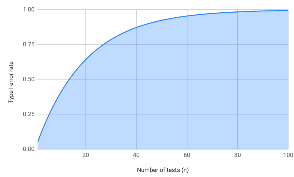
Any time we run a statistical test, the risk of a type I error equals alpha. So, in the example above, the probability that we incorrectly conclude AKT T308 expression differs between groups is 5%. Now consider that we’re rarely testing just one protein. Often we’ll compare the abundances of hundreds of proteins, if not more. When we run that many tests, the probability that at least one result is a false positive grows quickly, and can be quantified with the family-wise error rate formula 1−(1−α)ⁿ. Using this formula, we can see that with 1, 5, and 20 tests, the risk of at least one false positive is 5%, 23%, and 64%, respectively. By around 100 tests, the probability of at least one false positive approaches 100%, as you can see in the figure below. If we’re comparing hundreds of proteins or thousands of genes, false positives are essentially guaranteed.
The purpose of multiple testing correction is to reduce this risk of false positives as the number of tests increases. In practice, both the Benjamini-Hochberg and Bonferroni procedures accomplish this, but through different mechanisms and with different tradeoffs, as we’ll expand on below.
The Benjamini-Hochberg method controls the false discovery rate (FDR)—the expected proportion of false positives among all results we call significant. The procedure works as follows:
Rank all individual p-values in ascending order p(1) ≤ p(2) ≤ … ≤ p(m), where m in the number of statistical tests/comparisons we run.
Assign a rank i to to each ordered p-value, where i=1 is the smallest p-value and i=m is the largest.
Choose your acceptable FDR level (Q). A standard value is 0.05, meaning we tolerate up to 5% false positives among significant results.
Calculate the BH critical value corresponding to each p-value using the following formula: critical value = i/m * Q.
Find the largest p-value that is less than or equal to its corresponding critical value. That p-value and all smaller ones are declared significant.
As an example, suppose we’ve run 7 statistical tests and have the following ordered p-values: 0.01 ≤ 0.02 ≤ 0.04 ≤ 0.048 ≤ 0.05 ≤ 0.057 ≤ 0.06. Setting Q = 0.05, the BH critical values for ranks 1 through 7 are: 0.007, 0.014, 0.021, 0.029, 0.036, 0.043, 0.050. Comparing each p-value to its critical value, we find that none of the p-values are less than or equal to their corresponding critical value, so none of the results survive BH correction, despite several being below the naive p<0.05 threshold.
Using this method, you can see how the more tests you do, the harder it is for any given p-value to be significant after multiple testing correction. The chart below shows p-value rank plotted against critical thresholds. When m=2, the first (smallest) ordered p-value being significant at p<0.025, but as m increases we see this value getting smaller and smaller. By the time we reach m=6 we’re already at the point where p must be <0.01 to be significant.

The algorithm procedure above gives us a binary yes/no output for each tests—is it significant or not? The reason I introduced this first is that it helps build intuition for what BH correction is doing, but there is actually a simpler way to arrive at the same conclusion. One that produces a reportable adjusted p-value. To perform this method, we first rank order our p-values as we did previously, where p(1) ≤ p(2) ≤ … ≤ p(m) and m is the total number of tests. Then, for each of your p-values, use the following formula:
where i is the ordered ran and i=1 is the smallest p-value. However, after computing the adjusted p-value for all original p’s, we then apply a step-down forcing rule from the largest to smallest value to ensure the adjusted sequence never decreases as rank decreases. To definition for this rule as follows:
where you begin by applying the method to the largest p-value (called the base case) and work backwards to the smallest value. Using the same raw p-values as above, we now get the following results:
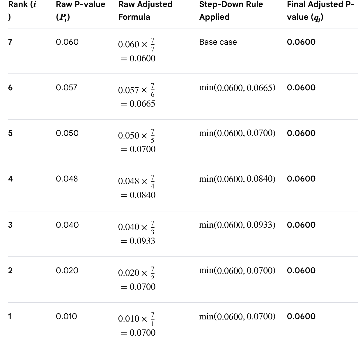
When the adjusted p-value (aka q-value) is smaller than our original α, then the adjusted p-value is significant.
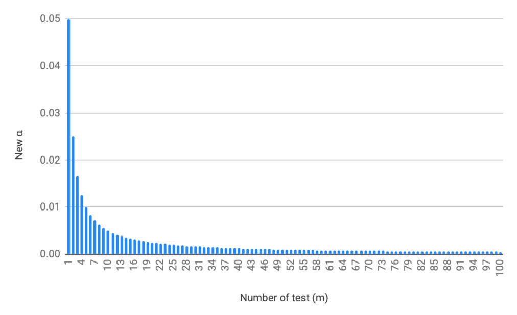
The Bonferroni procedure controls the family-wise error rate (FWER)—the probability of making even a single false positive across all tests performed. Rather than tolerating a controlled fraction of false positives as BH does, Bonferroni aims to ensure that the entire set of conclusions contains no false positives at all1. There are two ways to do this procedure, the first being the decision gate method, which scaled down the target significance (α) value based on the number of tests. To do this, we use the formula:
We then reject the null hypothesis for any test whose raw p-value is ≤ α_new. For example, with 20 tests and α = 0.05, the corrected threshold drops to 0.0025. With 100 tests, it drops to 0.0005, as you can see demonstrated in the chart below. As the number of comparisons grows into the hundreds or thousands—as is routine in proteomics and genomics—only the very strongest signals will clear this threshold. This makes Bonferroni highly conservative: it substantially reduces the risk of any false positive, but at the cost of a higher type II error rate (i.e., missing real findings).
Bonferroni correction can also be expressed as an adjusted p-value, which allows direct comparison to your original alpha. For each raw p-value, the Bonferroni-adjusted p-value is:
So, if your original p-value is 0.02 and m=10, our new p-value is 0.2. We can then compare this to alpha, where we get 0.2 > 0.05, therefore the result is not significant. Working backwards, you’d need a raw p-value of 0.005 or smaller to achieve significance at α = 0.05 with 10 tests—a demanding standard that grows more demanding with every additional comparison.
Whether you choose BH or Bonferroni comes down to what kind of error you’re more willing to tolerate. BH maximizes discovery—it finds more true positives, but accepts that some fraction of your significant results will be false. Bonferroni by contrast minimizes the chance of any false positive, but increases the risk of missing real effects.
For most exploratory bioinformatics analyses, BH is the appropriate choice. Proteomics and transcriptomics studies are typically hypothesis-generating, meaning their findings inform downstream validation efforts, not immediate clinical action. In this context, a false positive that gets filtered out in the next experiment is a manageable cost, and the greater statistical power of BH ensures you’re not missing real biology. There’s also an interpretive buffer built into pathway-level analyses: if AKT, mTOR, 4EBP1, and eIF4E all appear significantly elevated in TNBC non-responders, a single false positive among them doesn’t materially change the conclusion that the pathway is activated.
Our reasoning changes though when results directly inform clinical decision making. Imagine a clinical proteomics study identifying biomarkers to stratify patients onto different treatment arms in a cancer trial. A false positive in that context—a protein that appears to predict response but doesn’t—could result in patients receiving an ineffective or harmful treatment. Here, the acceptable false positive rate is not 5% of your hits; ideally it’s zero. Bonferroni correction, with its strict family-wise error rate control, is the appropriate tool when the downstream consequence of a single false positive is clinical harm rather than a failed replication.
Practically, we can use a simple heuristic to determine which test is appropriate: use BH for discovery-stage analyses where findings will be subject to further validation, and default to Bonferroni when results will directly inform clinical or regulatory decisions. This is the type of methodological judgment you don’t want an LLM to make for you. It doesn’t know whether your analysis is exploratory or consequential, or whether your hits will be validated in a follow-up experiment or used to stratify patients in a trial. When you prompt an AI to write your analysis pipeline, you need to supply that context and to do that, you need to understand the choice well enough to know it matters. That’s the irreducible core of what it means to be a computational biologist in the age of AI-assisted science.
Thanks for reading! If you found this post useful, please consider subscribing or sharing it with a friend. I regularly shared hands-on computational biology techniques, fresh ways to think about tough problems, and perspectives on a range of related topics.
This reflects a tension in statistical hypothesis testing: type I and type II error rates move in opposite directions. Reducing the probability of false positives (type I errors)—as Bonferroni does aggressively—necessarily increases the probability of false negatives (type II errors), meaning real effects that fail to clear the more stringent threshold go undetected. BH correction sits at a more permissive point on this tradeoff, accepting a controlled proportion of false positives in exchange for greater statistical power to detect true effects. There is no procedure that minimizes both error types simultaneously; the choice between BH and Bonferroni is ultimately a choice about which kind of mistake your scientific context can better tolerate.
Great explanation, thank you for the effort!