

Spectral Deviation From Randomness
Issue № 83 // Eigenvalue spectral deviation analysis, random matrix theory, and identifying candidate signatures of criticality


Issue № 83 // Spectral Deviation From Randomness
Principal component analysis (PCA) is a technique for finding the directions of maximum variance in high-dimensional data, transforming a set of correlated variables—for example, a bunch of protein’s expression levels—into a smaller set of uncorrelated features, or principal components. It’s for this reason that PCA is considered a form of dimensionality reduction, which is a jargony way of saying it reduces the number of input variables/features in a dataset while retaining as much information as possible. However, because PCA discards low-variance features it’s lossy, meaning you can’t reconstruct your original dataset after it’s performed. Instead, you’re left with a series of orthogonal principal components starting with PC1, which captures the highest variance, then PC2, PC3, and so on.
As a practical example, suppose we have a 200 x 1,000 matrix containing 1,000 protein’s expression values for 200 pancreatic cancer patients. This feature set exists in a 1,000-dimensional space, which is impossible to visualize, form a mental image of, or reason about directly.
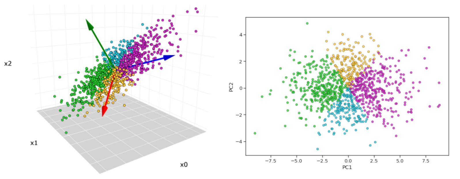
What PCA allows us to do is visualize this high-dimensional data in a low dimensional space—for example, compressing 1,000-dimensional proteomic data into just two ordered components that can be viewed via scatterplot (PC1 on the x-axis, PC2 on the y-axis). After running PCA we can also plot the cumulative variance explained per principal component, telling us how many PCs must be retained to preserve the majority of information from the original dataset. If just 20 principal components explain ~90% of the variance in our data, for example, it would allow us to work with just these 20 features per subject instead of 1,000, which is helpful for a number of reasons.1 Additionally, PCA can tell us whether our data actually has a low-dimensional structure, despite existing in a high-dimensional space, or whether it’s variance is diffusely spread across features, suggesting a more dilute signal (as is often the case in biology).
To this point, I’ve primarily been speaking about PCA from an information-centric perspective. Understanding that is step 1. What really confused me about principal component analyses even after I understood that though is what the principal components really represent. When we compress 1,000 protein’s expression values into a small handful of uncorrelated components, how should we think about these things? Additionally, if a given subject in our study has high level of PC1 compared to other subjects, what does that actually mean?
The easiest way to think about a principal component is as a weighted linear combination of all your original features. For easy math, let’s say we have 5 proteins in a dataset labeled proteins a-e. Each principal component score is a weighted linear combination of these features, which can be understood with the formula below where Zi is the 𝑖th principal component score, wij are the weights (aka loadings) for that component, and Xa...Xe are the original feature’s value (i.e., for each principle component, each sample gets a score determining how it’s projected onto that component in space).
When we run PCA, every protein in the dataset gets a unique loading value, or weight, for each principal component. This loading value indicates the degree to which that protein contributes to a given component and in which direction (positive or negative). If a protein has a high positive loading for PC1, it means that protein’s expression level is positively correlated with the PC1 score. Therefore, if a patient has high expression of that protein, the PCA algorithm calculates a positive score for them, moving them to the positive end of the PC1 axis. On the flip side, a protein with a high negative loading for PC1 is negatively correlated with the PC1 score. As a result, is a patient high abundance of that protein, they will be pushed towards the negative (opposite) end of the PC1 axis.
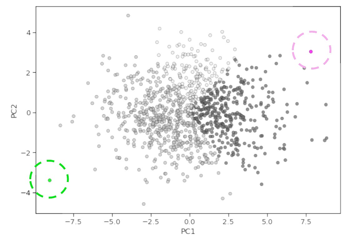
As previously mentioned, when used as a dimensionality reduction technique PCA removes redundancy in dataset by transforming correlated features into fewer, uncorrelated principal components while minimizing information loss. When used as an analysis tool though, it reveals underlying patterns in complex high-dimensional data by projecting them into simpler, easy-to-visualize spaces.
However, PCA has a limitation in that random noise has a structure—because PCA blindly maximizes variance it cannot distinguish between variance caused by a true biological signal, and variance caused by systematic structured noise. It’s for this reason that surrogate variance analysis is commonly used to identify and account for hidden batch effects and other unwanted sources or variation in multiomic data before performing PCA. But, what if we could use this unwanted variance to identify signs of criticality in our data?
If we filled a matrix with nothing but random noise, it’s eigenvalues (a measure of variance per principal component2) will not be zero—instead, they’ll form a predictable mathematical distribution.3 To extract real coordinated signals from data, we need to parse this baseline of noise and determine how a given dataset breaks from it. In random matrix theory, the Marchenko–Pastur (MP) distribution serves as the ultimate baseline, characterizing how the eigenvalues of a sample covariance or correlation matrix will behave if the underlying features have no true relationship and are driven purely by random chance. Rather than variance spreading uniformly, the MP distribution demonstrates that noise creates a bounded bulk of eigenvalues, with boundaries determined strictly by the ratio of features to observations. Consequently, any eigenvalue falling within these bounds is statistically indistinguishable from noise.
This is where eigenvalue spectrum analysis with spectral deviation comes in. Here, the “spectrum” is the complete collection of eigenvalues (one per principal component) generated from your data matrix. Spectral deviation is the metric that quantifies how drastically the empirically derived spectrum breaks away from the theoretical Marchenko–Pastur noise distribution. Eigenvalues that adhere to the MP curve suggest principal components pointing in directions of random fluctuation. Eigenvalues that pop out above the upper bound (λ>λ+) by contrast represent structural deviations. These outliers capture authentic, coordinated signals that defy random chance. By calculating this spectral deviation, we can strip away the illusion of structure created by noise, allowing us to accurately isolate the true underlying forces driving our system.
Before we dive into how eigenvalue spectrum analysis with spectral deviation can be used to identify signatures of criticality in our data though, we first need to cover the fundamental mechanics of how eigenvalue and vectors are calculated and what they mean. Let’s begin.
PS: there are a lot of footnotes in this piece. I recommend reading these if you get stuck with a concept as they provide important background and context.

A function f is a rule that maps each element in a set Α to exactly one element in a set Β. Therefore, for any element a in Α, we write f(a)=b, where b is the unique element in Β associated with a. For example, given the function f(a)=4a2, an input of 2 yield the coordinate pair (2,16). The set Α is called the domain of the function, and the set Β is the codomain. In this case, the inputs and outputs of the function are scalars.
When dealing with vectors, we use the vector spaces V and W to represent the domain and codomain respectively. Thus, we can view f as a transformation from V to W, which is expressed as f: V→W (this means “f maps V to W”).4 Here we are primarily concerned with linear transformations that take one n-dimensional input (x∈Rn ) vector and map it to an n-dimensional output vector (w∈Rn), which can be expressed as w=TA(x) or w=Ax. The transformation TA represents left-multiplication by A, where A is the standard n x n matrix. In the example below, TA: R2→R2 via multiplication by a 2x2 matrix.
When A is an n x n matrix, any non-zero vector x∈Rn is called an eigenvector of A if Ax is a scale multiple of x. In these cases, Ax=λx, for some scalar λ, where λ is the eigenvalue of A corresponding to the eigenvector of x.
Geometrically, an eigenvector represents a direction in space that maintains its orientation during a transformation; the vector is only scaled, stretched, or flipped along that specific axis5. The corresponding eigenvalue measures exactly how much scaling occurs. This geometric behavior directly underpins principal component analysis where the eigenvectors of a dataset’s covariance matrix identify the principal components (directions in protein space) and the eigenvalues then quantify the exact amount of variance traveling along each of those directions.
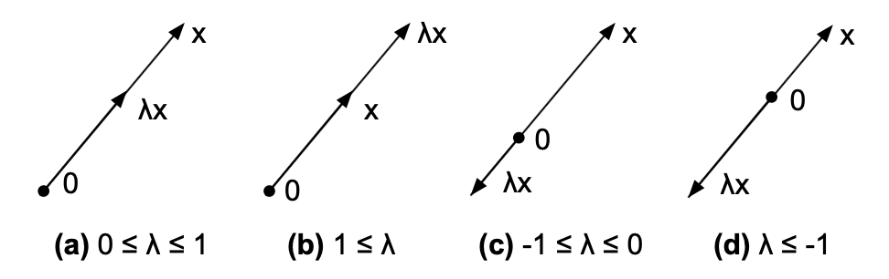
Below we demonstrate that a vector x is an eigenvector of standard matrix A with an eigenvalue (λ) of 3, by showing Ax=λx.
There are a handful of tricks you can use to calculate the eigenvalues and eigenvectors of an n x n matrix, but in practice it’s fairly tedious to do by hand for anything larger than a 3x3 matrix.6 As a result, we can solve for these variables with code, as demonstrated below.
A = np.array([[3, 0], [8, -1]]) # Define nxn matrix, A
eigenvalues, eigenvectors = np.linalg.eig(A) # Compute eigenvalues and eigenvectors
print("Eigenvalues:", eigenvalues)
# print("\nEigenvectors (columns):\n", eigenvectors)
Eigenvalues: [-1. 3.]You’ll note that the matrix above has two eigenvalues -1 and 3. An n × n matrix always has exactly n eigenvalues. Therefore, when generating a correlation matrix with n number of proteins, it will always have n eigenvalues with orthogonal eigenvectors.7
Now, imagine we have a 10x10 protein correlation matrix. Because it’s 10x10, it has 10 distinct eigenvalues ranked from λ1, λ2, …., λ10. These eigenvalues quantify the variance, and the total variance in the system is equal to the sum of the diagonal, which is always 10.0 in a 10x10 correlation matrix. If your first eigenvalue λ1 equals 4.2, then PC1 accounts for 4.2 units of variance, which if divided by the total number of proteins equals the percent variance explained. This means 42% of all protein fluctuations across your entire dataset can be explained by this single PC1 axis.
Each of the 10 eigenvectors itself contains 10 values called weights or loadings, which dictate how much each original feature contributes to the new direction. For example, if you look at PC1 it will contain a list of numbers—one for every single protein in your original dataset. For example, PC1 = [0.12, -0.45 ,0.78, …., 0.03]). When you project a data point onto this new PC axis, you calculate its new coordinate by multiplying each original feature value by its corresponding weight in the eigenvector, as demonstrated previously.
Now, recall earlier when I defined the eigenvalue spectrum as the complete collection of eigenvalues generated from your data matrix. Two facts make eigenvalues readable as a spectrum: first, the variance budget is fixed. The diagonal of a correlation matrix consists entirely of 1s, so the eigenvalues always sum to n (I.e., the modes, or PCs, divide up the fixed budget). Second, λ=1 is the natural baseline. If variance were spread evenly across all n directions, each mode would carry an eigenvalue of exactly 1. Therefore, an eigenvalue far above 1 indicates a direction along which many proteins move together far more than their fair share—a collective, coordinated mode. An eigenvalue below 1 on the other hand means that direction carries less than its fair share of the variance budget.
This ties into the Marchenko-Pastur distribution and why noise has a shape you can predict. Given n proteins that are completely independent from one another, we’d expect their correlation matrix to be the identity matrix, making all eigenvalues exactly 1 (the only eigenvalue for an identity matrix is λ=1). However, with finite samples, the off-diagonal correlations are never actually zero—two independent variables always show some spurious sample correlation when T (the sample size) isn't enormous. So, the empirical correlation matrix of pure noise is identity-plus-noise, and that noise smears the eigenvalues into a spread around 1.
Random matrix theory tells us exactly what that spread looks like. The Marchenko–Pastur distribution gives the eigenvalue density of a pure-noise correlation matrix, and it depends on the variable q, which is the ratio of observations to samples (i.e., proteins to patients). This distribution has hard edges (λmin and λmax), defined the following formulas.
Additionally, we can calculate the probability density function of the Marchenko-Pastur distribution, ρ(λ), which describes the behavior and distribution of eigenvalues for large sample covariance matrices using the formula below.
Statistically, the probability density ρ(λ) for λ>λmax is zero under the Marchenko-Pastur model and every noise eigenvalue falls between the λmin and λmax edges, meaning nothing pokes above λmax if the data is truly structureless.8 The code block below plots ρ(λ) against λ, demonstrating the distribution of eigenvalues relative to λmin and λmax. This relates to how we can use spectral deviation—departure from the MP null—as a criticality signal.
def spectral_dev(df):
  # calcualte correlation matrix; calculate eigenvalues
  corr_matrix = df.corr(method='pearson')
  eigenvalues, eigenvectors = np.linalg.eigh(corr_matrix)

  # derive MP edges; calculate p(lambda)
  q = len(df.columns) / len(df.index)
  lambda_max, lambda_min = (1 + math.sqrt(q))**2,  (1 - math.sqrt(q))**2
  grid = np.linspace(lambda_min, lambda_max, 500)
  mp_density = ((lambda_max - grid) * (grid - lambda_min))**0.5 / (2 * np.pi * q * grid)

  # plot ρ(λ) vs. λ
  plt.plot(grid, mp_density, color='red', label='Marchenko–Pastur')
  plt.hist(eigenvalues, bins=50, density=True, alpha=0.5, color='gray')
  plt.axvline(x=lambda_min, color='black', linestyle='--', linewidth=1, label=f'λ_min ({lambda_min:.2f})')
  plt.axvline(x=lambda_max, color='black', linestyle='--', linewidth=1, label=f'λ_max ({lambda_max:.2f})')
  plt.xlabel('Eigenvalues'), plt.ylabel('p(λ)'), plt.legend(), plt.show()
  return eigenvalues, lambda_max
eigenvalues, lambda_max = spectral_dev(df)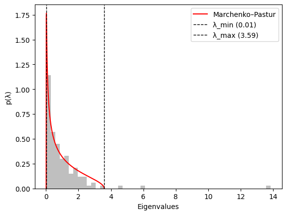
First, we can assess how many eigenvalues sit above the λmax edge, representing an axis of coordinated variation in the data. Counting these tells us the effective dimensionality of real underlying structure of the data.9 Additionally, we can calculate their variance share, which measures the percentage of total variance captured by these dominant eigenvalues relative to the variance of the remaining noise eigenvalues.
greater_lamba_max = np.sum(eigenvalues > lambda_max)
print('Eigenvalues > λmax:', greater_lamba_max)

var_share = round((np.sum(eigenvalues[eigenvalues > lambda_max]) / np.sum(eigenvalues[eigenvalues < lambda_max]))*100, 2)
print('% Variance Share for Eigenvalues > λmax:', var_share)
Eigenvalues > λmax: 3
% Variance Share for Eigenvalues > λmax: 25.31Second, we can observe the leading eigenvalue’s magnitude and how far it separates from the bulk (λ1 /λmax), called the spectral edge ratio.10 When a system is approaching a critical point—a loss of stability—it develops long-range, system-wide collective fluctuations. Here, many variables stop moving independently and start moving together. Spectrally, that collective coherence concentrates variance into a single mode, so λ1 swells and pulls far out past the edge, while a stable, well-behaved system spreads its variance across many modes and stays closer to the bulk.
spectral_edge_ratio = max(eigenvalues) / lambda_max
print('Spectral Edge Ratio (λ1/λmax):', round(spectral_edge_ratio,2))
Spectral Edge Ratio (λ1/λmax): 3.86While the spectral edge ratio tells us how strong the λ1 signal is, the normalized participation ratio (NPR) measures how that signal is distributed across the components of the first eigenvector (v1). The NPR maps the structural diffusion of the signal onto a strict scale: the closer the NPR is to its theoretical minimum of 1/N, the more localized the signal is within just one or two rogue components. Conversely, the closer the NPR is to 1.0, the more evenly distributed the signal is across all components. True criticality is ultimately confirmed when a high spectral edge ratio (such as the strong 3.86 deviation gap observed above) is paired with a high NPR, proving the transition is a diffuse, system-wide network phenomenon.11
What does this mean in practice? Suppose we have proteomic data from microdissected tumor samples collected after treatment and we want to compare criticality signatures between patients with a residual cancer burden of 1 (near complete pathological response) versus a residual cancer burden or 2-3. In this case, we might expect that treatment-resistant subpopulations show a more dominant leading eigenvalue and greater spectral edge ratio than a more sensitive subgroup. This could suggest the resistant clones have lost healthy regulatory boundaries, leading to a highly synchronized, single-minded survival state. However, depending on the experimental context the logic can reverse.12
The one big caveat here is that an inflated leading eigenvalue is consistent with criticality but is not proof of it. A single strong batch effect, a technical loading artifact, or one dominant biological covariate (proliferation, say) also produces one big eigenvalue. So, λ1 is a candidate signature that must be cross-checked against artifacts and against what its eigenvector actually loads on. If λ1’s eigenvector is uniformly high across all proteins, it’s likely a batch effect. On the other hand, if λ1 exhibits a high normalized participation ratio (NPR) driven by a highly correlated, diffuse network of diverse biological pathways, it is consistent with true criticality where the system undergoes a coordinated, collective state change (i.e., the majority of values in the eigenvector may be high, but to varying degrees) .
Notably, a signature of true biological criticality also dictates that the underlying proteins contributing to this high eigenvalue must also demonstrate an increase in variance across clinical conditions; for instance, if this critical signal is detected in non-responders, those participating proteins should display significantly higher variance than in responders. Conversely, if the signal is highly localized to just a few rogue components, it indicates a specific “core engine” pulling λ1 out past the noise edge—making it a potential therapeutic target rather than a global phase transition.
Thanks for reading! If you found this post useful, please consider subscribing or sharing it with a friend.
Many clustering algorithms, like k-means clustering, work better in lower dimensional space. A typical pipeline for clustering patients by protein expression is to z-score normalize proteins (column wise) to ensure they all contribute equally to the analysis regardless of their original scales, then perform PCA followed by k-means clustering. But, PCA isn’t always necessary (sometimes it’s even counter productive!). As a rule of thumb, PCA should be used before clustering when you have more features (proteins) than samples (patients), or when your data is noisy. So, for example, if you have 10,000 proteins and 500 patients, PCA makes sense. Technically, you don’t violate any statical assumptions or rules when using PCA in cases where samples >> features, but you do risk losing valuable signal by not preserving the full feature space.
Eigenvalues are scalars (constant numerical factors) used to scale an eigenvector. In the context of PCA, eigenvectors provide the weights (or loadings) used to compute the principal components, and eigenvalues explain the variance associated with a given PC. Given a scaled correlation matrix, the variance explained per principal component is its eigenvalue divided by the total number of features in the original dataset.
A matrix whose eigenvalues are all 0 is said to be nilpotent. Random matrices inherently avoid this due to probability; if you generate a random matrix , the odds of landing exactly on the knife-edge conditions that force every single eigenvalue to be zero are almost nonexistent. This implies that randomness has an underlying structure, and isn’t defined by complete chaos. In fact, when you analyze large random matrices distinct structures emerge, as predicted by random matrix theory.
A transformation is just a function, but the term of typically reserved for contexts like in linear algebra where the function alters the shape, size, direction, or scaling of a matrix or vector.
Relating this into PCA: Eigenvectors are principal components and they define the direction of the new axes. The values in the eigenvector are loadings, or weighs depending on whether they are scaled or raw. The eigenvalue corresponding to each eigenvector equals the variance of the data along that principal component axis (i..e, the variance explained per component). Finally, the PC score per sample is the linear combination of the sample’s original centralized values and the eigenvector weight.
According to the characteristic equation of an n x n matrix A, a scalar λ is an eigenvalue of A if and only if it satisfies the equation det(λI - A) = 0, where I is the identity matrix. This theorem provides a direct method for calculating the value(s) of λ. Additionally, a relative theorem states that if A is an n x n triangular matrix, its eigenvalues are the entireties of the main diagonal. Once we know the eigenvalues of a matrix, we can find its corresponding eigenvectors by solving for x in the equation (λI - A)x=0.
Here we use a correlation matrix instead of a covariance matrix since our features (protein measurements) have different scales. In effect, a correlation matrix is a covariance matrix that has been standardized to have a mean of 0 and a standard deviation of 1, ensuring all variables contribute equally to the analyses regardless of their original scales. In practice, this is why z-score normalization before PCA is standard with proteomic data.
When T ≫ N (q→0) and you have far more samples than proteins, both edges collapse to 1, making it much easier to distinguish signal from noise (i.e., the noise boundary is so tight, random noise can’t accidentally create large eigenvalues). On the flip side, when N ≈ T (q≈1), the band is wide and spurious structure is large. This has important implications when working with transcriptomic data, where often have few samples and many genes (N ≫ T). In these cases, several larger-looking eigenvalues could just be artifacts of the finite sample size rather than true biological signals and as a result we must use λmax to validate any real findings.
It also answers the question “how many principal components should I keep? Keep the ones above the MP edge, discard the rest as noise.
The purpose of quantifying spectral deviation in this context is to separate true, system-wide signals from sampling noise. In a finite system of uncorrelated variables, the MP distribution dictates that eigenvalues will naturally form a bulk bounded λmax. When measuring the spectral edge ratio a value of 1.0 is the absolute limit of random noise, which any value >1.0 directly scales with the strength of the emerging collective mode.
Importantly, you need to be sure that batch effects are not present before interpreting a large spectral edge ratio and NPR value as a sign of criticality. Because a batch shift alters many variables across a system simultaneously, it can synthesize a false collective mode. Therefore, confirming true criticality requires ensuring that the underlying data has been properly normalized to isolate true biological signals from technical confounding.
If measurements are pretreatment, the treatment-sensitive group is the one that typically exhibits criticality and a larger leading eigenvalue—suggesting the system is dynamically fragile and sensitive to therapy. Conversely, if the pre-treatment group has its variance spread across many smaller modes (staying closer to the Marchenko-Pastur bulk), it is a stable, well-behaved network—ie, therapy resistant.