Issue #69 // What Actually Makes Someone Good at ML in Computational Biology?

What separates good practitioners from great ones isn’t the code they write—it’s how they interrogate the output and what they bring to that interrogation that no automated pipeline can replicate.

Earlier this week I shared a new tutorial, How to Develop Predictive Biomarkers, which is designed to fill a conceptual gap—something I’ve identified when searching for resources that help computational biologists with intermediate machine learning experience leverage their unique skillset to create biomarker panels for predicting clinical outcomes (like treatment response in triple-negative breast cancer, for example).

Most existing resources cover isolated parts of ML model development, but none that I’ve come across explain the big picture—how the different parts of the pipeline fit together. This tutorial aims to do that, guiding you through the thinking process at each step from data acquisition to model deployment. Check it out, and please pass it along if you find it useful!

---

Issue № 69 // What Actually Makes Someone Good at ML in Computational Biology?

When I started building machine learning pipelines as a computational biologist, the whole thing felt suspiciously simple. End-to-end research projectsI’d worked on previously could easily rack up a few thousand lines of code. These pipelines? A few hundred lines, sometimes far less. This was incredibly confusing to me.

Source

After all, we’ve seen the news stories of AI researchers pulling multi-million dollar compensation packages. Surely there was more to it, right? The short answer is yes and no. In an interview with Dwarkesh Patel, Andrej Karpathy explains how neural networks can be built with just a few hundred lines of code.

"So micrograd is a 100 lines of pretty interpretable Python code, and it can do forward and backward arbitrary neural networks, but not efficiently. These 100 lines of Python are everything you need to understand how neural networks train. Everything else is just efficiency. […]There’s a huge amount of work to get efficiency. You need your tensors, you lay them out, you stride them, you make sure your kernels, orchestrating memory movement correctly, et cetera. It’s all just efficiency, roughly speaking. But the core intellectual piece of neural network training is micrograd. It’s 100 lines. You can easily understand it. It’s a recursive application of chain rule to derive the gradient, which allows you to optimize any arbitrary differentiable function." —Andrej Karpathy (source).

What commands a premium salary in a frontier AI lab isn’t just programming a model that works—it’s developing one that can be deployed and scaled to hundreds of millions of users with fractional efficiency gains at each step. That’s a whole other game entirely; one that demands deep expertise in computer science and AI.

This isn’t the game that biologists looking to utilize ML in their research are playing. A researcher who wants to build predictive biomarker panels, for example, needs to develop a much more narrow skillset. Additionally, after enough conversations with industry computational biologists I’ve come to the conclusion that what separates good practitioners from great ones isn’t the code they write—it’s how they interrogate the output and what they bring to that interrogation that no automated pipeline can replicate. Tommy Tang recently shared a post that perfect encapsulates this idea.

"Last week I asked Claude Code to highlight specific genes on a volcano plot. Simple request. The data matrix used Ensembl identifiers — those ENSG + 11-digit codes that map to specific human genes. I gave Claude Code the gene symbols I wanted highlighted. Instead of telling me it couldn’t map the symbols to Ensembl IDs, it fabricated identifiers that looked structurally valid. No error message. No warning. Just confidently invented gene IDs. I caught it for two reasons. First, I checked the mapping table. Second — and this is the part that matters — my positive control gene, one I know should be upregulated, was sitting in the wrong place on the plot. The biology didn’t make sense. Biology saved me. Not the AI." —Tommy Tang, Diving Into Genetics and Genomics.

So, as per the title, this issue will be about what actually makes someone good at applying ML to problems in computational biology. As always, if you find this post useful, please consider subscribing.

Integrating Domain Knowledge

In my opinion, the most important skill for a bioinformatics scientist or computational biologist isn’t their ability to code or do advanced math and statistics. It’s their ability to contextualize the outputs of their code and extract meaningful biological insights, which I previously wrote about in Issue #40: When Perfect Code Produces Imperfect Science.

Even something as simple as data cleaning, a foundational part of ML model development, requires a surprising amount of domain expertise. For example, when looking at proteomics data from 1,000 breast cancer patients you may notice that there are NaN values for ERBB2 (aka, HER2) across ~12% of the samples. Upon closer inspection, you see those samples correspond to patients classified as HR+HER2- and HR-HER2- via immunohistrochemistry (IHC), suggesting that missingness is due to ERBB2 expression being below the detection threshold of the assay used. Alternatively, suppose ERBB2 values missing, but with no clear separation by HR/HER2 status—in this case the NaN values may correspond to cases where there was not enough tumor sample to process (technical failure). These two cases should be handled differently and failure to so so could significantly impact downstream model performance¹.

This same principle applies to interrogating ML outputs. A pure machine learning practitioner looks at a LASSO output and sees features. A computational biologist looks at the same output and asks whether those features make sense.

• The bad version: "LASSO selected Protein X—let’s use it."

• The good version: "LASSO selected Protein X, but it’s a housekeeping protein that varies minimally across subjects and has no known connection to treatment response biology. Something’s off. Let’s investigate."

This kind of interrogation shows up at every step of the pipeline. It’s noticing that 15 of your 20 LASSO-selected proteins cluster into the PI3K/AKT/mTOR pathway, which either validates your model’s signal—for example, if your goal is to predict response to MK-2206, an experimental AKT inhibitor—or suggests it learned a single redundant axis dressed up as 15 independent features, suggesting it will fail to replicate in an independent patient cohort (for example, If your goal is to predict treatment response within a large TNBC patient population). Or, it’s flagging that your top predictive feature is a protein associated with sample preparation protocols at your institution (ex, Trypsin, albumin) rather than tumor biology—a pattern invisible to the code, but obvious to someone who knows their way around a wet lab.

Avoiding Overfitting—Including the Subtle Kinds

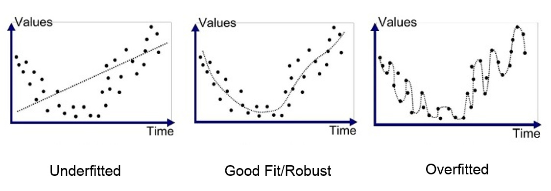
Overfitting is a modeling error in machine learning that occurs when a model learns training data too well, capturing noise and random fluctuations rather than just the underlying patterns. The most obvious form of overfitting—evaluating your model on the same data it was trained on—is easy to avoid once you know it exists. The subtle forms are where most people get into trouble.

Source

Implicit overfitting happens when you run multiple ML pipeline variations and report only the one that worked. Every time you run an additional experiment, you increase the probability that your good result is due to chance, whether or not you acknowledge it in the writeup. Metric overfitting, on the other hand, happens when you try several evaluation metrics and ultimately choose the one that best shows off your models performance. These actions don’t need to be intentional, nor do they always look like misconduct. However, they all produce the same outcome—results that don’t replicate.

What does good practice look like? Pre-specifying the full analytic approach before touching the data. This includes how you plan to clean and split the data, which feature selection method you’ll use and which algorithms you’ll spot check, how you’ll evaluate your performance, and what what count as success. This also means evaluating your final models performance once and reporting what comes out. Pre-registration, even informally in your own lab notebook, is dramatically underused in company biology and more valuable than most people appreciate.

Understanding Where the Model Fails

What does it mean to have a 3.75 GPA? Simply, it means that someone scored an A- on average. Without context that’s all we have to go off—maybe they literally pulled an A- in every class, maybe they got a B in some and A+ in others. You see, averages hide things. Similarly, an AUC (Area Under the Curve) metric averages a machine learning model’s performance, defined as the true positive rate, across all possible false positive rate thresholds. Typically, a AUC of ~0.8 or greater is considered quite good, particularly for predicting things like treatment response in diseases that lack clinically actionable biomarkers. However, evaluating a models performance based on a single metric can also be highly misleading.

• The bad version: "AUC is 0.81—ship it!"

• The good version: "AUC 0.81 overall, but 0.61 in the HR+/HER2- subtype. That’s the subtype we’d most want to spare from unnecessary chemotherapy. This model isn’t clinically useful for the patients it matters most for."

In clinical settings, the subgroup an ML model fails on is rarely random (this is another case where the ability to integrate domain knowledge separates a ML-first practitioner from a skilled computational biologist). It tends to be the subgroup with the least representation in training data, or the one where the underlying biology is most distinct, or both. A model with strong aggregate performance and a critical subgroup failure is often more dangerous than one with uniformly mediocre performance—because the strong aggregate creates confidence that isn’t warranted. Stratifying your confusion matrix by known clinical covariates—receptor subtype, disease stage, treatment arm—should be standard practice, not optional.

Handling Class Imbalance

Pathologic complete response (pCR) rates in triple-negative breast cancer range from ~30 to 60%. Treatment response rates in rare disease cohorts can be far worse, and in some adverse event predictions tasks there could be class imbalances of 100:1 or more². In these settings, a model that predicts the majority class for every patient will achieve high accuracy while being completely useless. For example, consider a dataset of patients with a rare autoimmune condition being treated with an experimental biologic. Of 400 patients, 360 are non-responders. If you built a model that predicts "non-responder" for everyone you’d be right 9/10 times. Saying we’ve achieved 90% accuracy is this case would be technically correct, despite the model learning nothing of value. The forty patients who might have benefited from treatment are invisible to it.

What’s the solution here? You could stratify splits, use a resampling method like SMOTE, or perform class weighting, among other options. The fixes here are usually straight forward, but it requires recognizing the problem first, which means looking at your class distribution before you look at performance numbers.

One practical heuristic: if you’re a biologist working on your first ML project and you’re achieving suspiciously good performance with minimal effort, look at your class distribution before you celebrate. Near-perfect accuracy on imbalanced data is one of the most common and least obvious failure modes in applied ML.

Knowing When to Stop

Of all the skills in this piece, knowing when to stop is the least discussed. The reproducibility crisis in clinical biomarker research is largely a consequence of implicit indefinite iteration: researchers modify their pipeline until the numbers look publication-worthy, then present the final result as if it were the first attempt. The forty previous iterations go undocumented and the published model looks clean and well-performing.

A model that achieves AUC 0.72 after a single pre-specified evaluation is more scientifically credible than one that achieves 0.85 after forty undocumented iterations. The former is a real signal. The latter might be—but you can’t know, and neither can anyone who reads the paper.

The habit worth building is simple: set your stopping rule before you start. Decide in advance what you’ll try, evaluate it once, and report what you find—including when it’s underwhelming. Frame modest results honestly, as a foundation for future work rather than a clinical breakthrough. This is what separates researchers who contribute durable knowledge from researchers who contribute noise. And it has nothing to do with how well you can write Python code.

1. For specifics on how you handle different types of missing data—depending on whether values are missing at random vs. not at random—you can check out Issue #63: When Absence Is Information—Missing Data in Proteomics.

2. Class imbalance occurs in machine learning when datasets have an unequal distribution of classes, where one majority class significantly outweighs one or more minority classes.