Issue #75 // An Intuitive Take on PCA For Biologists

What's the purpose of principle component analysis and what do principle components represent from a biological perspective?

Principle component analysis is a notoriously confusing topic for beginners in computational biology and applied ML. While the purpose of PCA—summarizing and compressing high-dimensional data—is relatively easy to understand, technical explanations are often overloaded with linear algebra, making them unwieldy and overwhelming. Personally, even after I had a firm grip on the math underlying PCA, I had trouble understanding what PCA was really doing to my data from a biological perspective. For example, after compressing 1,000 protein’s abundances into 30 principle components, what was I left with? More importantly, how should I reason about these abstract features when my ultimate goal is to cluster or classify patients? That’s what this article is about—providing an intuitive take on principle component analysis for biologists.

---

Issue № 75 // An Intuitive Take on PCA For Biologists

This article grew out of a simple question: practically speaking, what’s the purpose of principle component analysis (PCA) in computational biology and bioinformatics? The academic, and wholly unsatisfying, answer to this question is that PCA finds the directions of maximum variance in your data, transforming a set of high-dimensional correlated variables—for example, a bunch of protein’s abundances—into a smaller set of uncorrelated features, or principle components. For this reason, PCA is considered a form of dimensionality reduction, which is a smart sounding way of saying it reduces the number of input variables (features) in a dataset while retaining as much relevant information as possible. However, because lower-variance features are discarded, PCA is lossy, meaning you can never perfectly reconstruct your original dataset after it’s performed. Instead, what you’re left with is a series of orthogonal principle components starting with PC1, which captures the highest variance, then PC2, PC3, and so forth (we’ll come back to this shortly).

As a practical example, suppose we have a dataset with 50 protein’s values, each measured in an arbitrary number of breast cancer patients. This feature set corresponds to a 50-dimensional space, which while small in the grand scheme of bioinformatics analyses is impossible to directly visualize or reason about nonetheless. To make this concrete, imagine you wanted to visualize your heart rate data (a 1-dimensional data point) following a trail run. This could easily be viewed with a line graph. Now, let’s say you want to see two data points in relation to one another—heart rate vs. pace—this can be visualized on an x-y axis (i.e., a plane). Three? An x-y-z coordinate system. Anything beyond three dimensions though and we’re lost—our brains lack the ability to perceive a fourth spatial dimension and beyond, making it impossible to form a mental image of it.

Left: A 3D dataset where red, blue, and green arrows represent the first through third principle components, respectively. Right: Scatterplot after the data is reduced to 2 dimensions. (Image source).

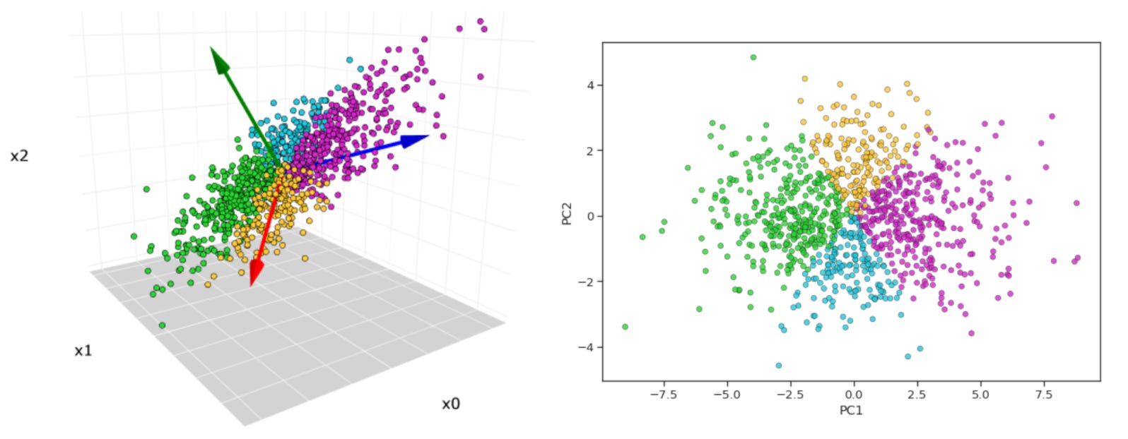
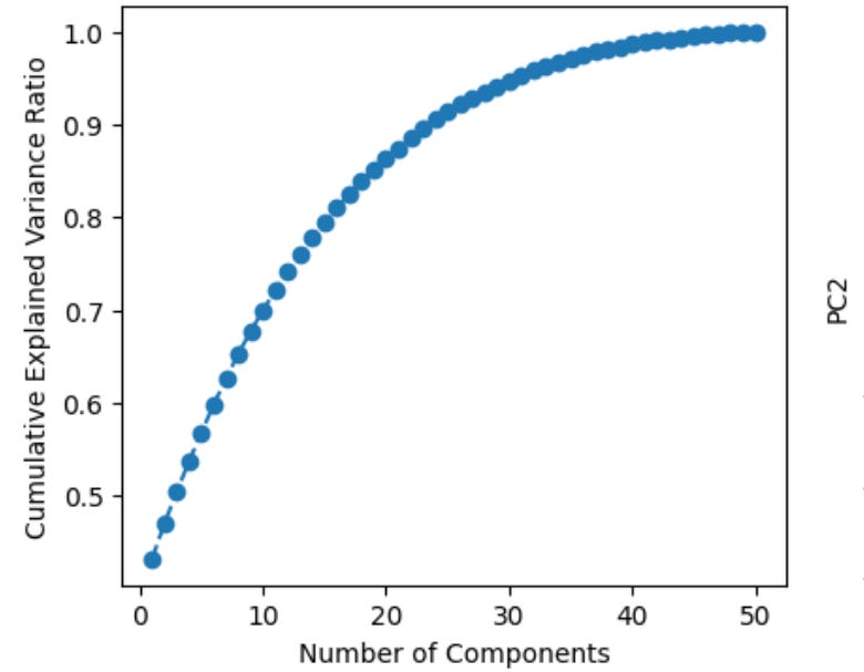
Now, what principle component analysis allows us to do is visualize high-dimensional data in a low dimensional space. For example, we can compress our 50-dimensional proteomic data into just a few ordered components that can be viewed in two dimensions (PC1 on the x-axis, PC2 on the y-axis). Additionally, after running this analysis we can plot the cumulative explained variance per principle component, which tells us how many PCs we need to retain the majority of information contained in the original dataset. Suppose we find that 20 components explains ~90% of the variance—this would allow us to work with just 20 features per subject instead of 50, which is helpful for a few reasons. First, many analyses downstream from PCA, such as k-means clustering, work better in lower dimensional space (see footnote #1 for a detailed explanation for when we should feed principle components into clustering algorithms and when we should use raw features instead)¹. Second, PCA can tell you whether our data actually has a low-dimensional structure, despite existing in a high-dimensional space, or whether it’s variance is diffusely spread across features, suggesting a more dilute signal (as is often the case in biology)².

Cumulative explained variance by PCA component.

To this point, I’ve primarily been speaking about PCA from an information-centric perspective. Understanding that is step 1. But, what really confused me about principle component analyses even after I understood the above is what the principle components really represent. When we compress 50 proteins abundaces’s into a small handful of uncorrelated components, how should we think about these things? Additionally, if a given subject in our study has high level of PC1 compared to other subjects, what does that actually mean?

Assuming you know some linear algebra, the easiest way to think about a principle component is as a specific weighted linear combination of all your original features. For easy math, let’s say we have 5 proteins in a dataset (labeled proteins a-e). Each principle component is a weighted linear combination of these features, which can be understood with the formula below where Zᵢ is the 𝑖-th principal component, wᵢⱼare the weights (aka loadings) for that component, and Xₐ..Xₑ are the original feature’s values.

\(Z_i = w_{i1}X_a + w_{i2}X_b + w_{i3}X_c + w_{i4}X_d + w_{i5}X_a + \)

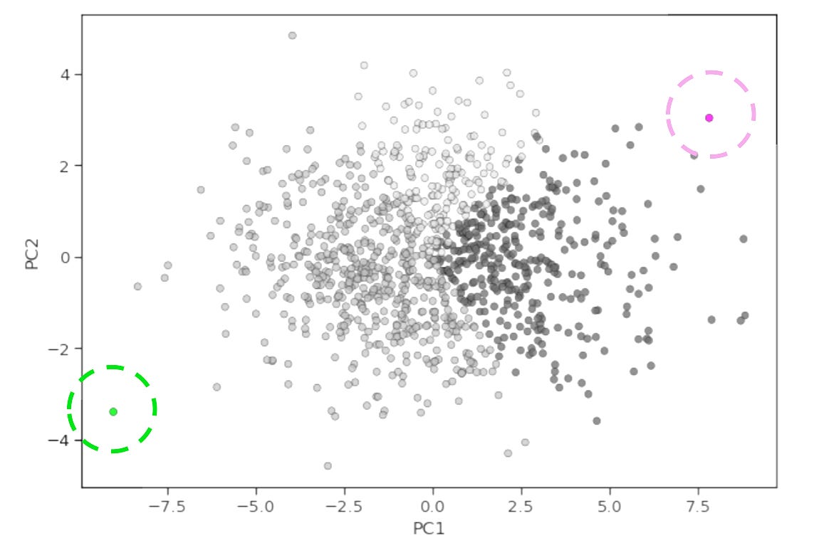
When we run PCA, every protein in the dataset gets a unique loading value, or weight, for each principle component. This loading value indicates the degree to which that protein contributes to given component and in which direction (positive or negative). If a protein has a high positive loading for PC1, it means that protein’s expression level is positively correlated with the PC1 score. Therefore, if a patient has high expression (high abundance) of that protein, the PCA algorithm calculates a positive score for them, moving them to the positive end of the PC1 axis. On the flip side, a protein with a high negative loading for PC1 is negatively correlated with the PC1 score. As a result, is a patient high abundance of that protein, they will be pushed towards the negative (opposite) end of the PC1 axis.

Patient 1 (green) has a high abundance of proteins with negative loadings for PC1 and PC2. Patient 2 (pink) by contrast has a high abundance of proteins with positive loadings for PC1 and PC2.

Now, if we take a specific linear combination of proteins (i.e., a principle component) we can determine whether it’s biologically meaningful by extracting its loadings. In simple terms, this is the weight of each protein in our original dataset for that component. We can then rank order proteins by their absolute loading values (while still being mindful of their direction) and ask “are the top contributes enriched in a particular pathway?” For example, we may see that PI3K/AKT/mTOR pathway proteins have high positive loadings for PC1, and immune checkpoint proteins have high positive loadings for PC2. This would indicate that the activation of the PI3K/AKT/mTOR signaling axis and the strength of immune checkpoint signaling are the two largest sources of variation in our data. From this, we might hypothesize that patients in the bottom right hand corner of a PC1 vs. PC2 x-y plot have the worst survival outcomes (high proliferation, low immune engagement) whereas those in the top left corner have the best survival (low proliferation, high immune engagement).

Alternatively, we may see that PI3K/AKT/mTOR pathway proteins have high positive loadings for PC1, and immune checkpoint proteins have high negative loadings for PC2, which would suggest that high PI3K/AKT/mTOR signaling and immune engagement are inversely associated in our data. Interrogating these types of outputs—rather than treating PCA as a push button analysis to be performed before clustering—is what sets a great computational biologist apart from the rest³.

Thanks for reading! If you found this post useful, please consider subscribing or sharing it with a friend. I regularly shared hands-on computational biology techniques, fresh ways to think about tough problems, and perspectives on a range of related topics.

1. This raises the question, when should we feed principle components into k-means clustering and when should we use raw features (protein abundance values in this example)? A typical pipeline for clustering patients by protein expression is to z-score normalize proteins (column wise) to ensure all of them contribute equally to the analyses regardless of their original scales, then perform PCA, then k-means clustering. But, PCA isn’t always necessary (sometimes it’s even counter productive!). As a rule of thumb, PCA should be used before clustering when you have more features (proteins) than samples (patients), or when your data is noisy. So, for example, if you have 500 proteins and 10000 patients, PCA makes sense. Alternatively, you should consider using raw scaled features when the number of proteins you’ve measured is modest relative to your sample size and you want to preserve the full feature space (ex, if you have ~100 proteins and patients both). Technically, you don’t violate any statical assumptions or rules when using PCA in cases where samples >> features, but you do risk losing valuable signals. A protein that contributes modestly to many principle components, but strongly to none, may never make it into your top PCs, despite potentially being the most clinically relevant feature. You can never know if you just compress it away unnecessarily. This is especially important to consider when using targeted proteomics panels, like reverse phase protein arrays where we often measure just ~150 proteins, yet may have hundreds or thousands of samples (as in large clinical trials, such as the ISPY-2 neoadjuvant trial).

2. Biological systems don’t actually operate in ~20,000-dimensional space, even though that’s how approximately many protein coding genes we can measure. The “true” dimensionality of biology may be orders of magnitude lower—perhaps hundreds of fundamental processes like immune response, cell cycle progression, or metabolic state that manifest through coordinated expression changes across thousands of genes and proteins.

3. For more on this topic, check out What Actually Makes Someone Good at ML in Computational Biology?