

Issue № 79 // Modeling Latent Variation in High-Dimensional Data
An in-depth guide to surrogate variable analysis (SVA) and what it can tell us from a dynamical systems perspective.


A quick PSA: After six years developing, validating, and commercializing a novel biosensing technology and optics platform, I’ve exited NNOXX. I’m now exploring opportunities in industry or academia where comp bio meets hard unsolved problems at the intersection of biology, AI, and complex systems science. If you’re working on something interesting, know someone who is, or just want to talk science, I’d love to connect (evanpeikon@gmail.com).

Issue № 79 // Modeling Latent Variation in High-Dimensional Data
In What Actually Makes Someone Good at ML in Computational Biology? I talked about the importance of handling class imbalance when developing a classifier to predict treatment response in triple-negative breast cancer. But, there’s another side to this that often goes undetected, especially in translational bioinformatics analysis. Imagine we wanted to compare the abundance of a specific set of signaling proteins and phosphoproteins between HER2+ and HER2- breast cancer patients. This seems relatively straightforward until you consider that HER2+ breast cancer tends to be diagnosed at a younger age on average compared to HER2-negative cases. Without age-balancing cohorts, we can easily introduce confounding variables into an experiment. The problem is these things aren’t always so easy to spot, which is where surrogate variable analysis (SVA) come in.
In Capturing Heterogeneity in Gene Expression Studies by Surrogate Variable Analysis Jeffrey Leek & John Storey state the following:
“In any given study there will be many other variables at play, such as the effects of age and sex on the disease. We show that in studies where the expression levels of thousands of genes are measured at once, these issues become surprisingly critical […] In any given study, it is impossible to measure every single variable that may be influencing how our genes are expressed. Despite this, we show that by considering all expression levels simultaneously, one can actually recover the effects of these important missed variables and essentially produce an analysis as if all relevant variables were included.”
SVA is a statistical inference technique that identifies and accounts for hidden batch effects and other unwanted sources or variation in multiomic data. It works by isolating unmodeled variation that is orthogonal (i.e., statistically independent) to the biological variables of interest. If you stratify patients by HER2 status (i.e., HER2+ vs. HER2-), for example, the assumption is that this variable affects a small portion of measured features (genes, proteins, etc.) and that factors likeage or BMI could be confounding your analysis. SVA uses that assumption to separate the desired biological signal from these latent technical variations1.
Despite SVA being able to attenuate batch effects, it is not itself a batch correction technique in that it doesn’t explicitly model known batch labels and remove their effect from a data matrix. In effect, SVA and batch correction tools like ComBat ask two different questions.
ComBat asks “Given that I know the batch labels, can I remove their effects from the data?” SVA, by contrast, asks “Given that something unmodeled is structuring my data, can I estimate what it is and account for it in downstream analysis?”
SVA accomplishes this by estimating surrogate variables (SVs), which are latent factors—things not directly measured, but whose influence you can detect in the things you did measure—that capture structured, unwanted, variation in data. It then includes those SVs as covariates in downstream statistical models (the linear model you run for differential expression analysis, for example)2. Notably, your data matrix is not modified when you do this as it would be with batch correction tools. Instead, the correction happens at the inference state. The implication here is as follows: after SVA, you do not get a corrected gene expression or protein abundance matrix. Instead, you get a set of surrogate variables that must travel with your data into whatever model you’re fitting.
As a rule of thumb, SVA fits in the stage of an analysis pipeline after you’ve performed basic normalizations and have log2 transformed your data, but before differential expression analysis with SVs as covariates. For gene expression data, this means that library size and depth should be account for prior to SVA. For reverse phase protein array data—what most of my recent work deals with—SVA is done after you’ve already performed dye-based normalization (i.e., Sypro Ruby loading normalization), calibration curve correction, and log2 transformation. A key concept here is that SVA needs data to be in a form where linear models are appropriate; log2 transformed data following the aforementioned normalization approaches accomplishes this. Running SVA on raw intensity values or pre-log2 transformed data would introduce errors; the heteroskedasticity in raw count-like data violates the linear model assumptions SVA relies on internally.
The best way to understand SVA and to develop an intuition for how it works is to break it into its component parts, then implement it from scratch. In practice, this means (1) regressing out the primary variable of interest (HER2 status, in this case) from each protein, then getting the residuals, (2) running singular value decomposition on the residual matrix to find the dominant axes of remaining variation, (3) determining how many SVs to retain, (4) including retained SVs as covariates in a downstream model.
To start, the following code generates synthetic reverse phase protein array data, which you can copy and paste into an IDE to follow along (for this tutorial assume that dye-based normalization calibration, and log2 transformation have already been performed upstream).
import numpy as np
import pandas as pd
np.random.seed(13)
n_samples, n_proteins = 200, 120
batches = ['B1','B2','B3','B4']
batch_assignments = np.repeat(batches, n_samples // len(batches))
her2_status = np.array(
    ['HER2+'] * 40 + ['HER2-'] * 10 +   # B1: 50 samples, confounded (HER2+ heavy)
    ['HER2+'] * 25 + ['HER2-'] * 25 +   # B2: 50 samples, balanced
    ['HER2+'] * 10 + ['HER2-'] * 40 +   # B3: 50 samples, confounded (HER2- heavy)
    ['HER2+'] * 25 + ['HER2-'] * 25     # B4: 50 samples, balanced)
data = np.random.randn(n_samples, n_proteins)
her2_effect = (her2_status == 'HER2+').astype(float)
data[:, :15] += 2.0 * her2_effect[:, None]   # true signal: first 15 proteins
batch_effects = {'B1': 1.5, 'B2': 0.0, 'B3': -1.5, 'B4': 0.0}
for i, b in enumerate(batch_assignments):
    data[i] += batch_effects[b]
protein_cols = [f'prot_{i+1}' for i in range(n_proteins)]
df = pd.DataFrame(data, columns=protein_cols)
df.insert(0, 'batch', batch_assignments)
df.insert(1, 'her2', her2_status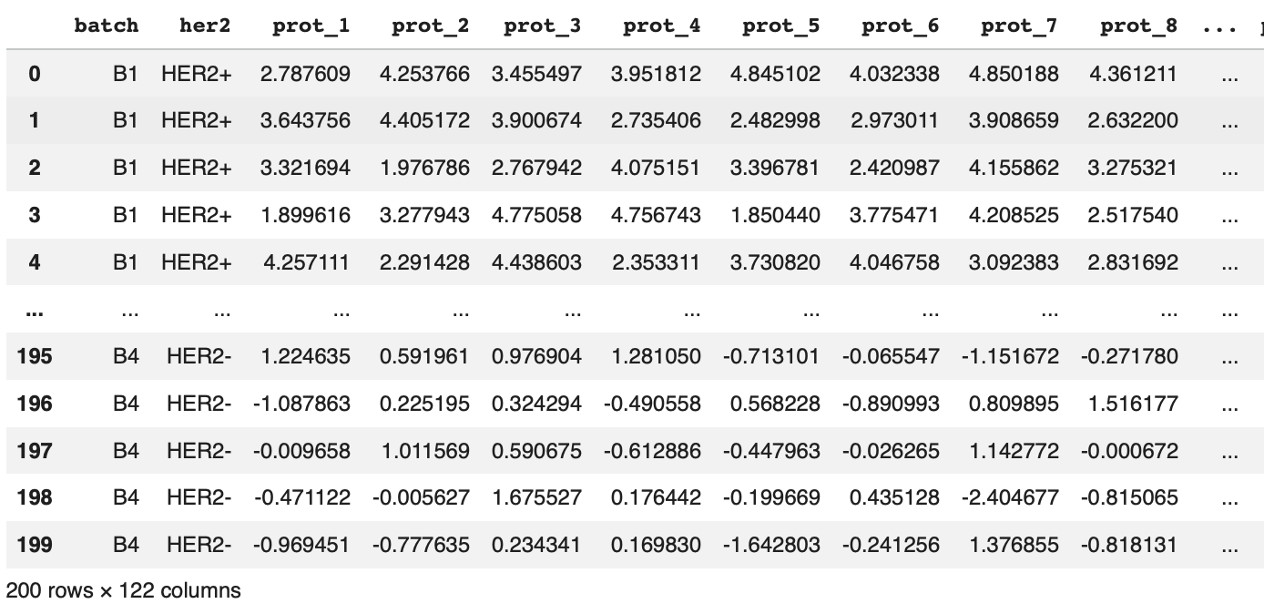
Step 1 — Regressing Out the Primary Variable
First, we need to regress HER2 status out of each protein’s expression vector, then take the residuals. Essentially, what we’re asking here is “what is the linear prediction of their protein’s expression given HER2 status?” The residual is then everything left over after that prediction is removed (i.e., the variation that HER2 status can’t explain). Once we do this for all 120 proteins in our synthetic dataset we end up with a 200 (samples) x 120 (protein) residual matrix with the HER2 signal removed from every protein column3.
Note: Performing SVD on this matrix finds the dominant axes of shared structure across proteins, which become surrogate variables. If we skipped this step and ran SVD on our raw data, the first singular vector would almost certainly capture the HER2 signal as that should be the largest source of variance in the dataset, and as a result we’d end up with a surrogate variable that partially represents the biology we’re trying to test (which is what we’re trying to avoid).
Regressing out a binary variable like HER2 status means we want to strip away any differences in protein levels caused by a patient being HER2+ or HER2-. In effect, cleaning the data so we can see what protein levels look like without the influence of HER2. To do this, we use the formula Protein level = Baseline Group Average + Group Difference + Leftover Info, which, is expressed as follows:
Here, the HER2 switch is either 0 or 1. Since we can’t put text into a math equation, we use a digital switch—if a patient is HER2-, the switch is 0 and if they are HER2+ the switch it 1. β0 is the y-intercept, which represents the average protein level for the HER2- cohort, and β1 is the slope which the difference you add or subtract if a patient is HER2+. Finally, ε is the residual or leftover protein level after we account for HER2 status—this is what we want to keep (i.e. the “HER2-cleansed” protein data).
Two questions you may have are (1) why is β0 the average protein level for the HER2- group? and (2) why is β1 the difference between the groups? When a patient is HER2-, their switch is 0. If we plug that into the equation we get protein = β0 + β1(0) + ε = β0 + ε. Therefore, β0 must represent the average protein level for the HER2- group, baring residuals. Additionally, when a patients is HER2+, their switch is 1. If we plug that into the equation above we get protein = β0 + β1(1) + ε = β0 + β1 + ε. Since we already know that β0 is the HER2- average, β1 has to be the exact distance/shift required to get from the HER2- average to the HER2+ average.
We can then calculate the residual by subtracting the predicted protein level (based on HER2 status) from the actual measured protein level for every single sample. For example, for a HER2- sample, the model predicts its protein level is exactly β0 and for a HER2+ sample, the model predicts its protein level is exactly β0+β1. Therefore, the residuals for HER2- and HER2+ samples are as follows: HER2- patient residual = (actual protein level) - (average protein level for HER- cohort) and for HER2+ patient residual = (actual protein level) - (average protein level for HER+ cohort). If we calculate a residual for all proteins and all patients, the residual is a 200x120 residual matrix, as mentioned above.
The code block below implements step 1 with two options: in the first example, I manually calculate the residuals and in the second I use statsmodels ordinary least squats (ols) function. Both give the same result.
'''Option 1: Manually Calculate Residuals'''
# Isolate HER2- and HER2+ patients into seperate dfs
her2_neg_list = df.index[df[’her2’]==0].tolist()
her2_neg_df = df[df.index.isin(her2_neg_list)]
her2_neg_df = her2_neg_df.drop(columns=[’batch’, ‘her2’])
her2_pos_list = df.index[df[’her2’]==1].tolist()
her2_pos_df = df[df.index.isin(her2_pos_list)]
her2_pos_df = her2_pos_df.drop(columns=[’batch’, ‘her2’])

# Calculate β0 and β1
B0 = her2_neg_df.mean(axis=0)
B1 = her2_pos_df.mean(axis=0) - B0

# Calculate residuals for HER2- and HER2+ patients
her2_neg_residuals = her2_neg_df - B0- (B1*0)
her2_pos_residuals = her2_pos_df - B0- (B1*1)

# Combine all residuals into a single df
residual_df = pd.concat([her2_pos_residuals, her2_neg_residuals], axis=0, ignore_index=True)

'''Option 2: Use statsmodels Ordinary Least Squares Regression'''
import statsmodels.formula.api as smf

df[’her2’]= df[’her2’].replace({’HER2-’:0, ‘HER2+’:1}) # Encode HER2-/+ as 0/1
residuals = []
for i in df.columns[2:]:
  model = smf.ols(f’{i} ~ her2’, data=df).fit()
  residuals.append(model.resid.values)
residual_matrix = np.array(residuals).T  # shape: 200 samples × 120 proteins
residual_df = pd.DataFrame(residual_matrix)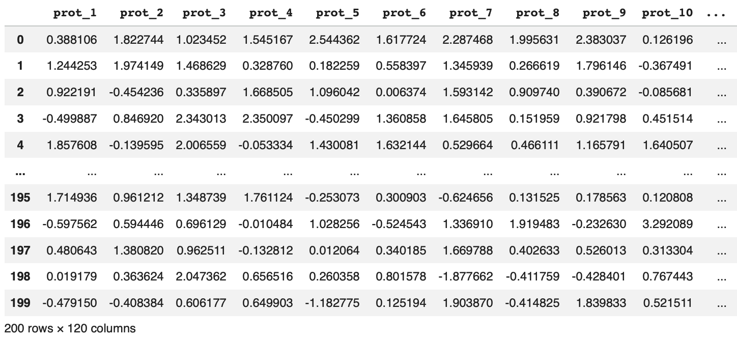
Step 2 — Singular Value Decomposition (SVD)
SVD asks, “what are the dominant axes of shared variation across proteins in the residual matrix?” Think of our 200 x 120 residual matrix as 200 samples sitting in a 120-dimensional protein space. Most of this space is noise—random, unstructured variation. But, if there are latent factors affecting many proteins simultaneously (i.e., a batch effect, processing artifact, or unrecorded clinical variable), the samples won’t be random scattered—they’ll be stretch along certain directions, or axes. SVD finds those axes, ranked by how much variance they explain. The decomposition gives three resultant matrices:
Note: Each latent factor explains something about the shared sample x protein space. The U matrix tells us how much of each latent factor (component) is in each sample, whereas the Vt matrix tells us how much each protein contributes to each latent factor. The end goal is to capture the dominant axes of variation, which means latent factors that collectively explain much of the variance in the shared sample x protein space.
U, which spans sample space, telling us how each sample loads onto each component. Since we have 200 samples, the full basis has 200 possible directions and therefore U is a 200 x 200 matrix (ie, each entry tell us how strongly that sample loads onto that component—directly analogous to PCA scores, which I’ve covered here).
Vt, which spans protein space, telling us how each protein loads onto each component. Because there are 120 proteins, the full basis has 120 directions and as a result Vt is an 120 x 120 matrix.
S, which contains singular values, one per component, representing the magnitude of each axis of variation. Because our S matrix can have at most min(200,120) non-zero singular values, the remaining 80 columns of U have no corresponding single value and carry no information about our data4.
Now, our surrogate variables come from the first few columns of U—one column per component we decide to retain. Each of these columns is a vector of length 200, gives every sample a score for that latent factor—this per sample score is what we include as a covariate in our differential expression model and it tells the model how much each sample was affected by that unknown factors. In order to decide how many columns of U (i.e., SVs) we retain, we look at S, which tells us how important each component is—components whose singular values are above what we’d expect by change are capturing real structure; the rest are noise5.
To perform SVD, we can use the following code:
# full_matrics=False gives "thin SVD" - only the 120 cols of U that have corresponding SVs
U, S, Vt = np.linalg.svd(residual_df, full_matrices=False)
After running this, we can then look at the distribution of singular values:
plt.figure(figsize=(12, 3))
plt.subplot(1, 2, 1), plt.plot(S, marker='o', linestyle='-'), plt.grid(True)
plt.title('Distribution of Singular Values'), plt.xlabel('Singular Value Index'), plt.ylabel('Magnitude')
var_explained = S**2 / np.sum(S**2)
cum_var_explained = np.cumsum(var_explained)
plt.subplot(1, 2, 2), plt.plot(cum_var_explained, marker='o', color='orange')
plt.title('Cumulative Variance Explained'), plt.xlabel('Number of Components'), plt.ylabel('Proportion of Variance')
plt.grid(True), plt.tight_layout(), plt.show()
In the left plot we see that the first singular value (149.6) is dramatically separated from the rest, then there’s a sharp drop down to 24.1 followed by a smooth decay. The right plot shows that this first component explains ~50% of the residual variance after we regressed out the primary variable (HER2 status) in step 1. Now, recall from the synthetic data generate code block that we intentionally skewed batch composition, with batch 1 being HER2+ heavy and batch 3 being HER2- heavy. Knowing this, we can logically assume that this first surrogate variable is a batch effect. Additionally, we can see that the remaining components decay gradually without an obvious second elbow, suggesting that the nature of remaining variation may be noise with no additional latent structure (this is what we’d expect from this synthetic dataset where batch is the only intentional confounder). This brings us to step 3.
Step 3 — Determining How Many SVs to Retain
In the last step we performed SVD, giving us a vector of singular values. This leads directly to the retention decision—deciding how many SVs to keep before building them into our DE model. There are three common ways for doing this:
The elbow method, where we retain components about an obvious break (the plot above has one clear break after the first component).
Using a variance threshold, where we retain components until we hit some cumulative variance explained, like 80%. In the chart above we can see this occurs around 40 components.
Performing a permutation test, where we permute the residual matrix, recompute singular values, and retain components whose observed singular value exceeds the permuted null.
Of these, the elbow method is fast and often defensible, then the break is clean as in the case above, but it requires judgement and there is some arbitrariness involved. Variance thresholds are equally arbitrary—the 80% convention has no biological grounding. As a result, I tend to err towards permutation testing when it’s not abundantly clear how many SVs should be retained. The permutation tests is the most principles choice as it generates an empirical null, asking not “how much variance does this component explain?” but “does this component explain more variance than you’d expect by chance if there were no latent structure?”
Essentially, a permutation test works as follows: if you shuffle the rows of different protein columns randomly, you destroy any latent structure in the data while preserving the marginal distribution of each protein. SVD on that permuted matrix gives you a null distribution of singular values—what you’d see if there was nothing there whatsoever. We then repeat this many times, then retain components from our original SVD whose observed SV exceeds the 95th percentile of the null.
n_permutations = 1000
null_singular_values = np.zeros((n_permutations, min(residual_df.shape)))

# Permutation loop — store null singular values
for i in range(n_permutations):
  shuffled_data = np.apply_along_axis(np.random.permutation, 0, residual_df) # Shuffle each column independently using NumPy
  _, S_permutations, _ = np.linalg.svd(shuffled_data, full_matrices=False) # Run SVD
  null_singular_values[i, :] = S_permutations

# Compute 95th percentile of null for each component
null_95 = np.percentile(null_singular_values, 95, axis=0)

# Check which singular values pass the 95th percentile
passed_sv = S > null_95
n_passed = np.sum(passed_sv)
print(f"Number of Singular Values passing the 95th percentile: {n_passed}")
Number of Singular Values passing the 95th percentile: 1
Now, recall that our surrogate variables are stored in the columns of U (one column per component we decide to retain). Since we’re only retaining one component, we can access it via U[: , 0], which we’ll use in the next step.
Step 4 — Including Retaining SVs as Covariates in Downstream Analyses.
The final step is to include our retained SV as covariates in our downstream statistical models—in this case differential expression analysis. Here, we’ll be fitting a per-protein linear model of the form protein ~ HER2_status + SV1, which tells us the difference in protein expression between HER2+ and HER2- patients, after holding SV1 constant.
df['SV1'] = U[:, 0] # Add SV1 to data frame
parameters = [] # OLS coefficient for HER2 status
p_vals = []
for i in df.columns[2:-1]:
  model = smf.ols(f'{i} ~ her2 + SV1', data=df).fit()
  parameters.append(model.params['her2'])
  p_vals.append(model.pvalues['her2'])
adjusted_p_values = stats.false_discovery_control(p_vals, method='bh')
log2FC = df[df['her2']==1].iloc[:,2:-1].mean(axis=0) - df[df['her2']==0].iloc[:,2:-1].mean(axis=0)
results_dict = {'Protein': df.columns[2:-1], 'HER2- Mean':df[df['her2']==0].iloc[:,2:-1].mean(axis=0), 'HER2+ Mean':df[df['her2']==1].iloc[:,2:-1].mean(axis=0),
                'Parameters':parameters, 'log2FC':log2FC, 'p-val':p_vals, 'Adj. p-val':adjusted_p_values}
results_df = pd.DataFrame(results_dict).set_index('Protein')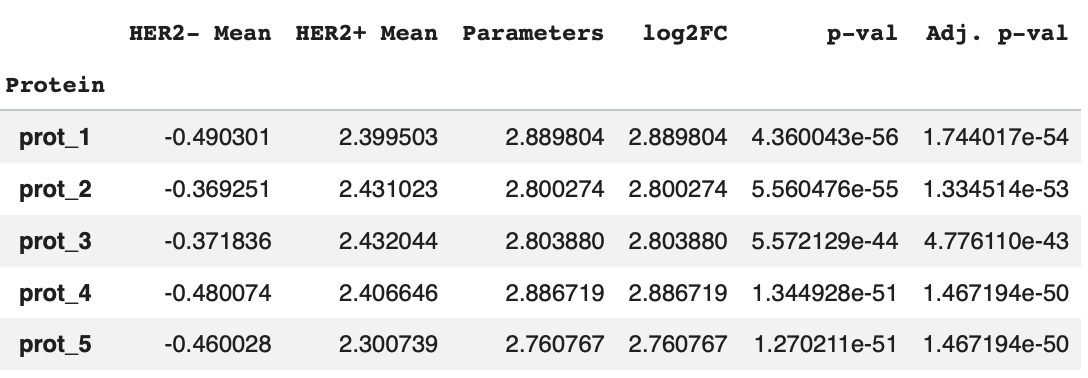
Because HER2 is encoded as 0/1, the coefficient in the "Parameters" column above is interpreted as: for a one unit increase in HER2 status (i.e., going from HER2- to HER2+), protein expression changes by this many units on the log2 scale, after accounting for the latent factor captured by SV1. This is directly comparable to the more common log2FC effect measurement in DEA, but the difference is that whereas log2FC is the raw mean difference between groups, ignoring SV1, the parameters in our OLS model (below) is the HER2 effect after partialling out SV1.
A Dynamical Systems Perspective on SVA
Note: If this section is of interest, make sure to check out Issue 80, which will be a deep dive on resolving attractor geometry from high-throughout proteomic data.
Observing the number of dominant axes of structured variation in proteomic state space tells us a lot about where a population sites relative to attractor states. In the case above, we have one dominant axis of residual variation after regressing our HER2, meaning the remaining structure is essentially one-dimensional. This is consistent with a single latent factor, batch, pulling samples along a one-dimensional sub-manifold in protein space (“sub”, because the full dominant structured variation is two-dimensional when accounting for HER2 status).
In this light, batch effects aren’t just statistical nuisances. They are geometric distortions of the state space you’re trying to study. When PCA separates samples by batch versus biology, the dominant axis of the empirical space is technical versus biological. The attractor structure you actually care about—whether your conditions are truly distinct stable states with a high energy barrier between them, or whether they are on a continum—is invisible because the batch manifold is overlaid on top of it. SVA’s job is to collapse that technical dimension so the intrinsic geometry of the biological landscape becomes recoverable. Therefore, performing PCA post SVA is the first look at the actual shape of biological state space you’re working in. Two tight, well-separated, clusters suggests bistabilty—two distinct attractor basins with a high barrier between them (a third cluster that falls outside either group may represent a subpopulation occupying an intermediate or alternative attractor state, often corresponding to a transitional phenotype). Substantial overlap suggests a single broad attractor with your condition of interest varying continuously.
Similarly, after correction, bimodal protein expression distributions become interpretable as biology rather than artifact. A single protein with two peaks across the patient population suggests a bistable regulatory node—a switch-like gene where the system stably occupies either a high or low state with an unstable intermediate. These are candidate drug targets because pushing them from one state to the other produces a qualitative change in system behavior, not just a graded response. Bimodality that appears after correction but not before is a direct example of SVA recovering attractor geometry that batch distortion had obscured.
Thanks for reading! If you found this post useful, please consider subscribing or sharing it with a friend. I regularly shared hands-on computational biology techniques, fresh ways to think about tough problems, and perspectives on a range of related topics.
Notably, this method fails when your primary variables does in fact affect the majority of measured features, which can occasionally happen when (a) measuring a small-ish number of features or (b) using a high-targeted proteomics panel, such as reverse phase protein arrays. I’ve written about this previously in Bypassing Stability Assumptions in High-Throughout Proteomics.
SVA is incompatible with non-parametric methods, such as Wilcoxon rank sum tests. Instead, it is used with parametric methods, like linear regression, t-tests, and ANOVA, for example. As a result, high-throughout proteomic data should be log2 transformed to stabilize variance and linearize the data before use with SVA and downstream analyses.
What remains is a mixture of true technical noise, latent structured variation (batch effects, processing artifacts, unknown confounders), and any biological variation unrelated to HER2 status (for example, hormone receptor status).
The last 80 columns of U are mathematically valid basis vectors but are composed of pure noise. They exist to make U a square matrix, not because they represent anything meaningful in your data.
Vt tells you which proteins are driving each component. This is useful for biological interpretation but not needed for the covariate adjustment itself. As a reference, looking at Vt loadings in SVD is conceptually similar to looking at PC loadings in PCA, and if your data matrix is centered before SVD, the rows in Vt are identical to the same PC loadings you’d get from a standard principle component analysis.