

Anticipating Cascading Failures in Complex Adaptive Systems
Issue № 85 // Identifying critical slowing down with matrix decomposition and classic statistical inference. An in-depth guide.


Note: This issue is a bit math heavy in parts, but those details are not necessary to understand the piece overall. I’ve also included over a dozen extensive footnotes with additional background information to help clarify difficult to grasp concepts. However, if you have questions feel free to ask them in the comments section or via my contact form.
Issue № 85 // Anticipating Cascading Failures in Complex Adaptive Systems
Complex adaptive systems from financial markets, to the human proteome, and even ecosystems can have tipping points where the system abruptly shifts from one state to another. These shifts are exemplified by diverse phenomena including sudden global financial market crashes, malignant cellular transformation in oncogenesis, and local ecosystem collapse—the latter of which has been famously demonstrated in the Peter Lake Study, providing the first real-world evidence that ecosystems take longer to recover from small shocks just before major cascading failures occur.1
Predicting these transitions is notoriously difficult because complex adaptive systems seldom present visible signs or symptoms before a tipping point. Additionally, mechanistic mathematical models of these systems often lack the granularity needed to pinpoint where exactly these critical thresholds reside in state-space (i.e., the theoretical landscape of all possible configurations the system can experience). There are, however, certain generic warning signals that appear across a wide array of systems approaching critical points, and to the extend that we can measure the state of these systems (via sensors or otherwise), these signals can be utilized to anticipate critical transitions before the threshold is breached. It may seem strange that disparate phenomena—the collapse of an over harvested tuna population and a wild swings in a companies stock price, for example—display similar signals, but the same general mathematical properties do in fact describe various systems near critical point independent of their specific physical details.
One of the most telling clues for identifying when a system nears a critical threshold relates to a concept in dynamical systems theory called critical slowing down (CSD), which is characterized by a system’s decrease in the rate of return to equilibrium following a perturbation, shock, or stressor. The most obvious implication of this phenomenon is that if we were to experimentally perturb a system—say, by adding or removing a small number of top predators to an ecosystem—we could subsequently measure it’s recovery rate to determine how close it is to a bifurcation point (an area in state-space where a small change in conditions causes a sudden runaway change in the system’s behavior).
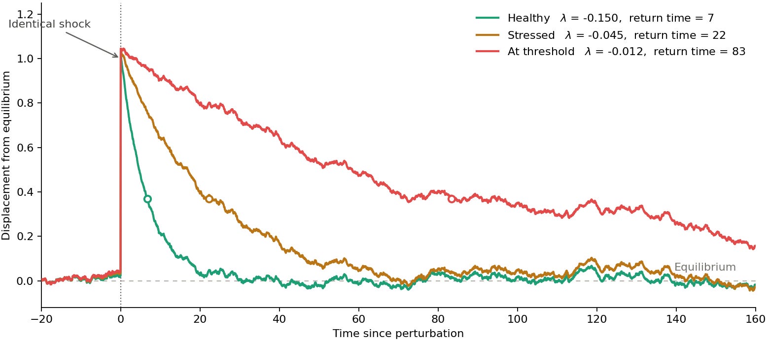
Of course, systematically testing recovery rates is both unethical and impractical for the majority of natural systems. However, for modeling purposes, almost all real-world systems are subject to natural environmental perturbations and we can use these background fluctuations and shocks to understand the system’s characteristic changes that subsequently occur. For example, as a bifurcation approaches, we should expect CSD to result in increasing auto-correlation defined as the degree of similarity between a system's current state and its state at a previous time step. While this is intuitive to understand—slowing down causes the intrinsic rates of change to decrease, and as a result the system’s state at any given moment increasingly resembles its past state—it can also be demonstrated mathematically.
The Jacobian Matrix As an Indicator of Critical Slowing Down
Mathematically, CSD occurs when a the dominant eigenvalue of a system’s Jacobian matrix moves closer to zero. The Jacobian matrix is a grid of all first-order partial-derivatives of a vector-valued function which is a rule that maps a coordinate vector of input variables (x1, x2,…,xn) to a set of output functions, where each input variable has its own governing differential equation.2
In a complex adaptive system, each sub-function (f1, f2,…, fn) represents the rate of change for a specific variable over time and the Jacobian is the best local linear approximation of the non-linear system near a specific point, demonstrating how a small change in any input variable scales and impacts every output variable simultaneously.3 Given a system with n variables (x1, x2,…,xn) and n equations (f1, f2,…, fn), the Jacobian is structured as follows.4
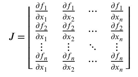
The eigenvalue of the Jacobian matrix represents the system’s restoring force; when a perturbation pushes the stable system away from equilibrium, a large negative eigenvalue acts like a string spring pulling the system back quickly. As the system approaches a critical transition though, its underlying stabilizing mechanism weakens. Here, the dominant eigenvalue of the system’s Jacobian matrix drifts from a negative value towards zero (λ → 0), representing a loosening of its internal “spring.” Because the restoring force is nearly gone, the system can no longer quickly erase the impact of random external shocks and therefore the effect of a perturbation from yesterday lingers into today, and today’s state influences tomorrows, and so forth—it’s for this reason that critical slowing down is associated with increased variance.5
While the Jacobian matrix is considered a foundational tool for explaining why CSD occurs, constructing it requires knowing the explicit differential equations governing the system you’re studying. When working with real-world data, we almost never known these underlying equations—as a result, we can’t construct a Jacobian matrix. Instead, we need to rely on statistical early warning signals within our data itself. For example, given a time-series from we can build a trajectory matrix, which is a formed by stacking time-lagged vectors for a single continuous time-series to reconstruct a system’s phase space.
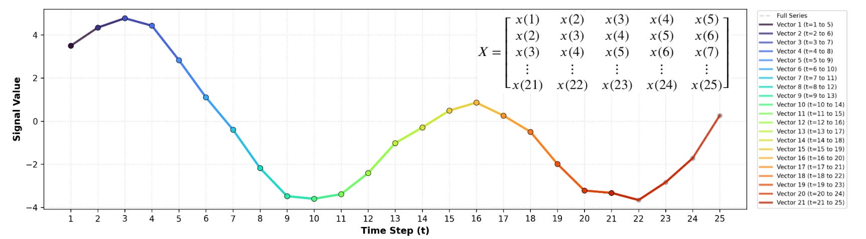
Whereas the Jacobian matrix provides continuous eigenvalues, the trajectory matrix of a time-series provides discrete values. Thus, the statement “critical slowing down is associated with eigenvalues moving towards zero” refers strictly to the eigenvalues of the Jacobian matrix. When working with a trajectory matrix, we instead see the leading discrete eigenvalue increase from 0.0 towards 1.0 as the system approaches a bifurcation point, reflecting increased remembrance of its past. To detect this empirically, we can apply principal component analysis (PCA) to the trajectory matrix—a method formally known as Singular Spectrum Analysis (SSA).
Detecting Hidden Dynamical States with Singular Spectrum Analysis
Standard PCA is traditionally applied to multivariate data, where columns represents different observed variables (ex., protein expression), rows represent samples, and all features are measured at the same time point. In this context, each principal component is an eigenvector (representing a direction in space that maintains its orientation during a transformation) in state-space composed of loadings, which describe the degree to which each feature contributes to that specific principal component.6 Additionally, the eigenvalues quantify the variance associated with each principal component.
With SSA, by contrast, PCA is applied to a single time series in the form of the time-lagged trajectory matrix which reconstructs a multi-dimensional proxy phase space. When we run PCA on this trajectory matrix, it’s resultant eigenvectors are called temporal principal components (or temporal empirical orthogonal functions), representing the time-dependent patterns of dominant waveforms of the system’s dynamics. The corresponding eigenvalues for each temporal principal component in turn represents the statistical variance or energy contains within each temporal component.7
To translate this information into an early warning system we need to analyze time-series data across two distinct temporal scales: chronological time (to observe shifts over the experiment’s duration) and lag time (to measure system memory within a specific window). In practice, this requires slicing a long time series into localized chronological segments and then constructing a Hankel matrix inside each segment through the following multi-step workflow: first, we perform chronological slicing by partitioning a long continuous time series in rolling or adjacency blocks.
For example, if we have a series containing 40 observations, we can segment it into four sequential blocks of 10 observations each where block 1 spans from t1 to t10, block 2 spans from t11 to t20 and so on (in reality, 40 observations is far too short of a time-series or this analysis, but it makes for easy visualization below). This step establishes a macro-timeline to evaluate whether the system’s proximity to a tipping point increases from one block to the next.
After segmenting our time-series into blocks—which are effectively isolated flat vectors—the second step is to construct the Hankle matrix (lag space), transforming each block into a multidimensional matrix to reveal its internal dynamics. Within each block of N observations (here N=10) we select a window length (L), which dictates the lag-depth of the matrix.8 In this case, we’ll select a lag-depth value of L=5. By sliding the window across the N points, K= N-L+1 time-lagged vectors are generated and stacked. The genetic format for the Hankle matrix is featured below.
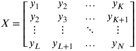
Now, for a worked example, with N=10 and L=5, K is equal to 6. Thus, we expect to have four separate 5x6 matrices (X1, X2, X3, X4) with 5 rows and 6 columns. The first of these matrices X1 is visualized below. T
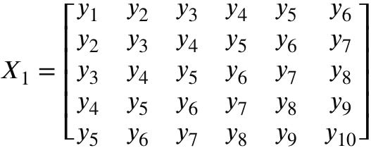
Notice that within the Hankle matrix all elements along the anti-diagonals (i.e., the diagonal lines running from the bottom-left to top-right) are identical. This step mixes space and time through lagging, allowing the analysis to capture how long the memory of past perturbations lingers inside that specific block. After obtaining the Hankle, we next generate the lag-covariance matrix, which we get by multiplying each Hankle matrix by its transpose (XXT). For a Hankle matrix with dimensions LxK, this operation results in a LxL matrix as demonstrated below for X1X1T.9

Within the lag-covariance matrix, the rows and columns no longer map to sequential chronological time stamps; instead, they represent distinct lag dimensions. Consequently, this matrix directly quantities the lag-covariance of the system (hence the name), which explains how a time-series of data relates to a delayed version of itself.
Finally, once we have a lag-covariance matrix corresponding to each chronological block, we can extract their individual eigenvalues, allowing us to quantify the total statistical variance (or energy) contained within the specific dynamical patterns and waveforms found inside the corresponding time period. If the underlying system we’re measuring is experiencing critical slowing down we should expect λ1 block 1 < λ1 block 2 <…< λ1 block n, signaling that the system’s physical restoring forces are weakening.10
Because variance skyrockets along the specific axis of failure, the leading eigenvalue of the lag-covariance matrix swells massively from one time block to the next while it’s corresponding eigenvector maps the exact geometric path or waveform of the impending collapse. In practice, this means the system sheds its complexity and compresses its dynamics into a single, dominant, low-frequency oscillation (similarly to how the ocean recedes and organizes into a single, massive, wave at the shoreline prior to a tsunami). As as result, instead of tracking dozens or hundreds of independent physical variables, it’s possible to monitor just this leading eigenvalue—using it’s sudden surge in energy—to forecast the timing and pattern of systemic failure before it occurs.
Now, in the code block below you’ll find a worked example for how to segment a time-series into blocks, how to convert each block into a lag-covariance matrix (LCM), and how to extract the leading eigenvalue from each LCM.11
def SSA(df, num_blocks=10, lag_depth=0.5):
  len_df = len(df)
  N = len_df//num_blocks
  L = int(N * lag_depth)
  K = N-L+1
  hankels, covs, eigvals, eigvecs = np.zeros((num_blocks, L, K)), np.zeros((num_blocks, L, L)),  np.zeros((num_blocks, L)), np.zeros((num_blocks, L, L))

  for i in range(num_blocks):
    block = df['x_csd'].iloc[i*N : (i+1)*N].to_numpy()
    block = block - block.mean()
    for l in range(L):
      hankels[i, l, :] = block[l : l + K]
    covs[i] = hankels[i] @ hankels[i].T / K
    w, v = np.linalg.eigh(covs[i])
    eigvals[i],eigvecs[i] = w[::-1],v[:, ::-1]

  lead_eigval = []
  for i in range(num_blocks):
    print(f"block {i+1:2d}  λ1={eigvals[i,0]:8.4f}  λ2={eigvals[i,1]:8.4f} λ1+λ2={eigvals[i,0]+eigvals[i,1]:8.4f}")
    lead_eigval.append(eigvals[i,0])

  sns.set_theme(style="darkgrid")
  sns.lineplot(x=range(1, 11), y=lead_eigval, marker='o', color='crimson', linewidth=2)
  plt.fill_between(range(1, 11), lead_eigval, color='crimson', alpha=0.2)
  plt.xlabel('Chronological Block'), plt.ylabel('λ1'), plt.title('Leading Eigenvalue of Lag-Covariance Matrix Over Time')
  plt.show()
  return None

SSA(df, num_blocks=10, lag_depth=0.5)
block 1 λ1= 1.3177 λ2= 1.1622 λ1+λ2= 2.4799
block 2 λ1= 1.0259 λ2= 0.8442 λ1+λ2= 1.8701
block 3 λ1= 0.4879 λ2= 0.4685 λ1+λ2= 0.9564
block 4 λ1= 1.2081 λ2= 0.7928 λ1+λ2= 2.0009
block 5 λ1= 0.3755 λ2= 0.3688 λ1+λ2= 0.7443
block 6 λ1= 1.0567 λ2= 0.6464 λ1+λ2= 1.7031
block 7 λ1= 1.9565 λ2= 1.0375 λ1+λ2= 2.9940
block 8 λ1= 0.5944 λ2= 0.5057 λ1+λ2= 1.1002
block 9 λ1= 0.5179 λ2= 0.4481 λ1+λ2= 0.9661
block 10 λ1= 5.7944 λ2= 5.5935 λ1+λ2= 11.3879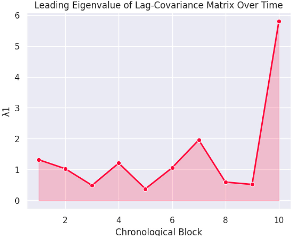
Capturing Spatiotemporal Patterns with Multivariate Singular Spectrum Analysis
In practice, singular spectrum analysis requires us to know which measurement is most useful to monitor ahead of time. Since we can’t count on that being the case, we can instead scale this approach to complex, multi-variable datasets—such as tracking hundreds of distinct protein abundances simultaneously. Here, we transition from univariate SSA to multivariate singular spectrum analysis (MSSA) where instead of analyzing a single data stream, we capture the spatiotemporal patterns of a system by evaluating how different physical variables interact across both chronological time and lag time.
To implement MSSA we start with chronological slicing and normalization. First, we partition a long parallel time series of all variables (features) into matching temporal blocks—for example, segmenting a 100-point timeline for 500 proteins into synchronized blocks of 25 observations. Because different physical variables often operate on entirely different scales, it’s important to z-score normalize each time-series feature column individually within each block, ensuring that a single high-abundance protein does not artificially dominant downstream variance calculations, for example.
Next, we construct a block trajectory matrix. With isolated blocks of N observations, we select a shared window length of L for all features, then construct individual LxK Hankel trajectory matrices fore each feature using the standard lagging method where K=N-L+1. For a system tracking multiple variables (ex, protein A and protein B), we stack these individual matrices within each time block to form a block trajectory matrix, x̃. Given M variables, x̃ will have the dimensions (MxL)xK. By stacking the data this way you force the algorithm, to look across different physical systems simultaneously.
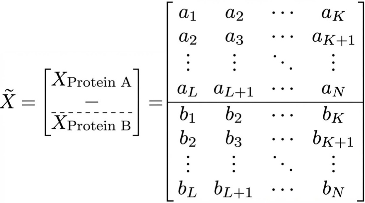
After generating the block trajectory matrix, we multiply it by its transpose (x̃x̃T), yielding a square matrix with the dimensions (MxL)x(MxL)—the rows and columns of the resultant matrix represent cross-lag covariance, a measure of how a change in one variable at an earlier time relatives to a different variance at a later time, mapping dynamical dependencies across the system.
Finally, we can extract eigenvalues from the square cross-lag covariance matrix for each block. In a healthy system, individual components fluctuate randomly and independently, spreading statistical variance evenly across a flat-ish spectrum of many small eigenvalues. However, as a system approaches a tipping point, CSD forces independent variables to lose their operational freedom causing individual sub-types to phase-lock and move together in synchronized waves. By running the MSSA pipeline block by block, we can track leading eigenvalues (λ1) across time, assessing the height, power, and coordination of system-wide waves. When the leading multichannel eigenvalue explodes, it’s signals that the overarching physical forces stabilizing the entire network have broken down. Meanwhile, if you were to have just looked at raw protein expression levels, you will often see absolutely nothing change before a collapse. Many systems maintain a steady mean value right up until they hit a bifurcation point. By calculating the leading eigenvalue across sliced blocks, you are tracking a hidden mathematical transition (this is true whether you’re looking at protein abundances, stock prices, or other measurable indicators of a systems state).
Classical Statistical Methods for Identifying Critical Slowing Down
While matrix decomposition methods like SSA and MSSA offer structural views of system collapse, they are not the only ways to detect this transition. Orthogonal signatures of critical slowing down can also be identified using simpler classical statistical methods. Because the weakening of the Jacobian eigenvalue reshapes the system’s entire frequency spectrum, this increased memory can be measured in several ways from patterns of fluctuations in time-series data. The simplest approach is to track lag-1 autocorrelation, which is a proxy for the slowness of recovery following natural perturbations.
In a healthy system, the effects of random shocks are erased almost instantly, meaning the systems state at time ti tells you little to nothing about its state at time ti+1 (i.e., there is low auto-correlation). As the continuous eigenvalue of the Jacobian drifts towards zero though, the system losses its elasticity and shocks from yesterday begin to linger into today—causing the time series to become highly predictable from one moment to the next. This results the lag-1 autocorrelation metric climbing steadily towards 1.0 as the tipping point approaches.
Another inevitable consequence of critical slowing down Is an increase in variance within the patterns of fluctuation. This behavior can be formally proven (see footnote #5), but it’s also intuitive to understand through the lens of accumulating shocks: as the Jacobian eigenvalue approaches zero, the impact of external disturbances no longer decays. Instead of being neutralized by a strong internal force (a large negative λ value), the uncorrected shocks pile up over time, inflating the variance of the state variable. As a result, even if the absolute baseline mean of a system’s measurements remain flat, the amplitude of it’s background noise will expand, providing a clear statistical indicator of impending collapse.
Before lag-1 autocorrelation and variance can be calculated, the data needs to undergo a preprocessing step called detrending—the process of removing long-term systematic variations, trends, or mean changes from time-series or sequential data. CSD discovery metrics are designed to measure short-term noise fluctuations around a system’s local equilibrium; because real-world biological or environmental systems often exhibit slow, long-term shifts in their baseline mean feeding raw trend data directly into autocorrelation and variance calculations will cause our models to mistake slow changes the underlying data for CSD—introducing false positives.
To isolate fast-acting noise fluctuations from long-term trends, we apply a rolling mean subtractor to extract clean residuals using the formal below, where yt is the raw data point and μrolling(t) is the local average calculated within a moving window centered at time t.12 All subsequent early warning statistics are calculated exclusively on these flattened residuals.
The evaluate these indicators over time, we analyze rolling blocks of a single time-series y=[y1, y2, …, yn] using the following definitions: first, lag-1 autocorrelation (ρ1) is measures how strongly a system’s current state correlated with it’s immediate past. As the system slows down, it’s memory deepens, driving this value towards 1.0.13
Sample variance (σ2) by contrast measures the spread of the data points around their mean. As the system’s restoring force weakens, uncorrelated shocks add up causing this value to expand.
By plotting these statistics across chronological blocks. we can observe signatures of criticality. For example, imagine that in window 1 (healthy) we see a ρ1 value of 0.031 and in window 45 (CSD) ρ1 spikes to 0.486. This would indicate that the system’s memory has increased, reflecting a weakened restoring force. Similarly, when this occurs we may see σ2 trending upward as noise accumulates and global variance begins to skyrocket.
In the code block below I’ve provided a worked example for these concepts using the same synthetic dataset from the earlier SSA example.
DETREND_WIN, WIN, STEP = 100, 100, 5
def detrend(s, window=DETREND_WIN):
    mu = s.rolling(window, center=True, min_periods=1).mean()
    return s - mu

def rolling_ews(resid, win=WIN, step=STEP):
    v, idx, rows = resid.to_numpy(), resid.index.to_numpy(), []
    for a in range(0, len(v)-win+1, step):
        w = v[a:a+win]
        rows.append(dict(centre=idx[a+win//2], ac1=np.corrcoef(w[:-1], w[1:])[0, 1], var=w.var(ddof=1)))
    return pd.DataFrame(rows).set_index("centre")

def kendall_tau(y):
    y = np.asarray(y, float); n = len(y); c = 0.0
    for i in range(n-1):
        c += np.sign(y[i+1:] - y[i]).sum()
    return c/(0.5*n*(n-1))

def surrogate_p(resid, stat="var", n_surr=500, seed=0):
    x = resid.to_numpy() - resid.to_numpy().mean()
    phi = np.corrcoef(x[:-1], x[1:])[0, 1]
    sd  = x.std()*np.sqrt(1-phi**2)
    obs = kendall_tau(rolling_ews(resid)[stat])
    rng = np.random.default_rng(seed); null = np.empty(n_surr)
    for k in range(n_surr):
        y = np.empty(len(x)); y[0] = rng.normal(0, x.std())
        e = rng.normal(0, sd, len(x))
        for i in range(1, len(x)):
            y[i] = phi*y[i-1] + e[i]
        null[k] = kendall_tau(rolling_ews(pd.Series(y, index=resid.index))[stat])
    return obs, (null >= obs).mean()

mu, resid    = df.x_csd.rolling(DETREND_WIN, center=True, min_periods=1).mean(),  detrend(df.x_csd)
ews   = rolling_ews(resid)
tau_ac1, tau_var = kendall_tau(ews.ac1), kendall_tau(ews['var'])
fig, ax = plt.subplots(3, 1, figsize=(10, 8), sharex=True)
ax[0].plot(df.index, df.x_csd, lw=.7, color='0.5', label='raw')
ax[0].plot(df.index, mu, lw=1.6, color='black', label='rolling mean')
ax[0].legend(); ax[0].set_ylabel('x')
ax[1].plot(df.index, resid, lw=.7, color='darkgreen'); ax[1].set_ylabel('residual')
ax[2].plot(ews.index, ews.ac1, color='red', marker='.', label=r'$\rho_1$')
ax[2].set_ylabel(r'$\rho_1$', color='red'); ax[2].set_xlabel('t')
ax2 = ax[2].twinx()
ax2.plot(ews.index, ews['var'], color='blue', marker='.', label=r'$\sigma^2$')
ax2.set_ylabel(r'$\sigma^2$', color='blue')
plt.tight_layout(); plt.show()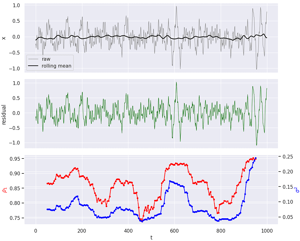
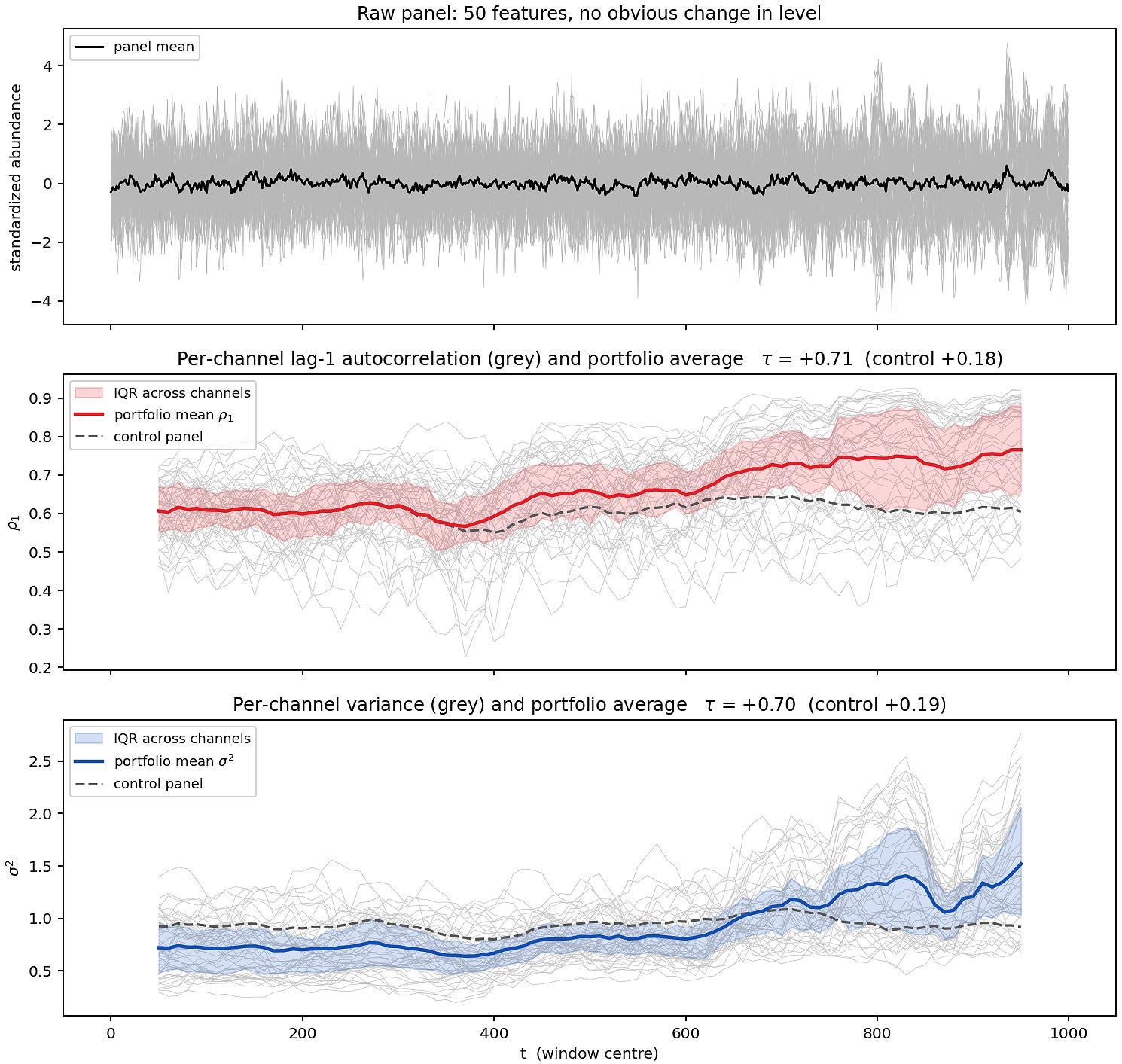
Because these metrics are done for each time-series variable in a multi-metric dataset individually (ex, a 50 protein time series) we end up with separate variance curves and auto-correlation curves over time. To make sense of this massive volume of individual metrics, we can aggregate signals using one of three standard methods: first, we can use the portfolio averaging approach where we calculate the average variance and autocorrelation across all channels for each time block. As a system tipping point approaches, we should expect the mean autocorrelation and variance of the system to drift upwards, as you can see demonstrated in the image below.
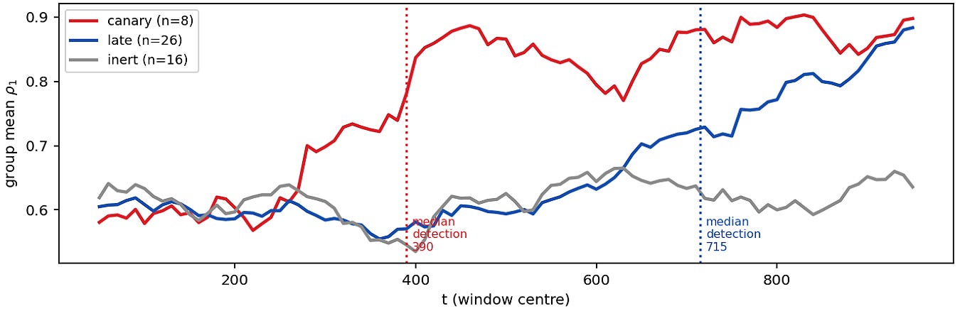
The second approach is the canary in the coal mine; here, we look for a specific subset of features whose variance and autocorrelation explode first. Because the master Jacobian eigenvalue affects variables differently based on network topology, certain specific feature will display critical slowing down much earlier than others, acting as early warning beacons.
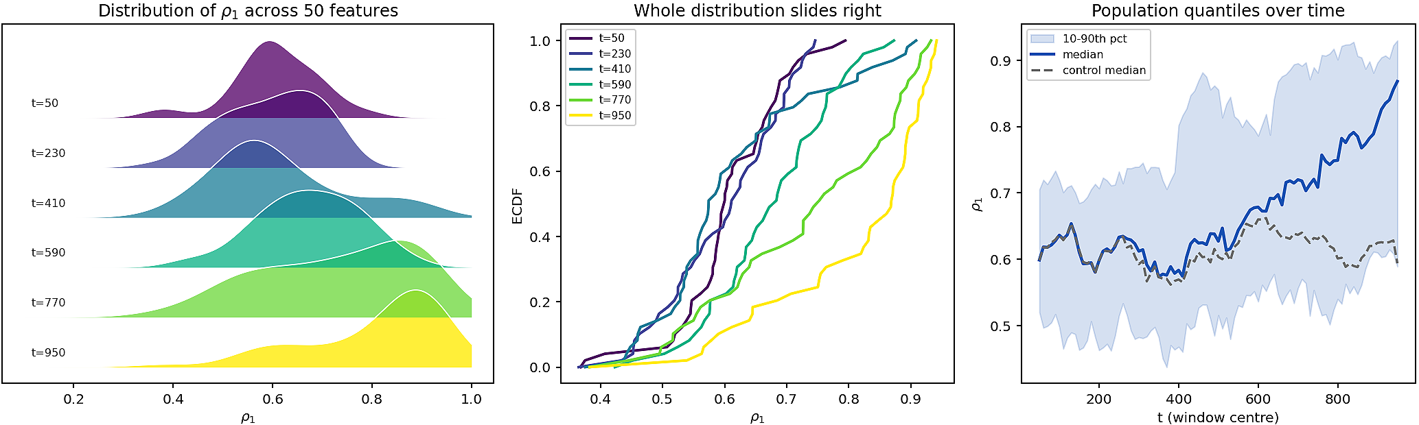
The third and final approach is to look at distribution shifts, which we can do by plotting a histogram of the autocorrelation values for all of our features proteins in window 1 vs window 2 … vs window n. As criticality nears, you will see the entire distribution skew heavily to the right, showing that the vast majority of individual measurements are simultaneously losing their restoring forces.
Practical Takeaways — My Personal Preferences
Classic statistical inference approaches to identifying critical slowing down—like variance and lag-1 autocorrelation—are useful in that they are highly sensitive and easy to compute, but they have limitations in that the resultant signals are both noisy and local. Singular spectrum analysis and MSS by contrast handle noise well; yet, they are inventive to raw magnitudes of chance. In practice, this means we need hybrid approach that blends matrix decomposition and classical statistical methods. My personal preference is to start by running a rolling window variance and lag-1 autocorrelation calculation across all features in a dataset, then looking at the portfolio average and distribution shift. If I see that across the population of features, autocorrelation is climbing and that variance is expanding it signals to me that CSD may be occurring somewhere in the system. From here, I use MSSA to isolate the signal.
Because univariate metrics are noisy, we can’t rely on them alone to forecast the shape of system collapse. By feeding high-dimensional time series data into MSS and calculating the leading block-covariance eigenvalue we can determine where and when λ1 begins to swell and break away from lower eigenvalues, exceeding the random noise threshold—this indicates that the aforementioned statistical signals are not random noise and that the system is syncing up into a singular, coordinated wave. Finally, we can extract the loadings from the leading eigenvectors, telling us which subset of features are “vibrating” together on this frequency, which we can use to determine which part of the system is going to break.
Thanks for reading! If you found this post useful, please consider subscribing or sharing it with a friend. I regularly post hands-on computational biology tutorials and perspectives on a range of topics.
Natalie Wolchover wrote a great piece on this study for Quanta Magazine titled Nature’s Critical Warning System.
A vector-valued function only outputs a single value for each equation and as a result it’s represented by a column vector. The Jacobian is a grid matrix because it takes every single equation (each row in the vector-valued function) and differentiates it against every single variable (each column).
A vector-valued function is non-linear if its output functions contain variables that are multiplied together, raised to powers, etc. In complex systems, this means variables interact dynamically rather than changing at constant, predictable rates. By definition, a purely linear system cannot be a complex adaptive system because linear systems are predictable and proportional—a small change always produces a small predictable response. Complex adaptive systems by contrast require non-linear interactions to generate their defining traits, such as emergence, self-organization, feedback loops, and sudden tipping points.
For a worked example, let’s take a simple system where…
The generic format of the Jacobian for this system can be characterized as follows:
Now, if we take the partial derivative of dx1/dt with respect to x1 and x2 we get 2x1 and 1 respectively (Note: if you’re unfamiliar with partial derivation and want to learn more, check out Math for Computational Biology). If we take the partial derivative of dx2/dt with respect to x1 and x2 we get 3 and -2x2. Therefore, the assembled 2x2 Jacobian matrix is as follows:
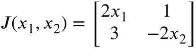
We can then evaluate the Jacobian matrix at specific coordinates by plugging in values for x1 and x2 as desired to get the constant matrix, whose eigenvalues we can assess as mentioned above. Because they describe a continuous-time system, these eigenvalues are continuous.
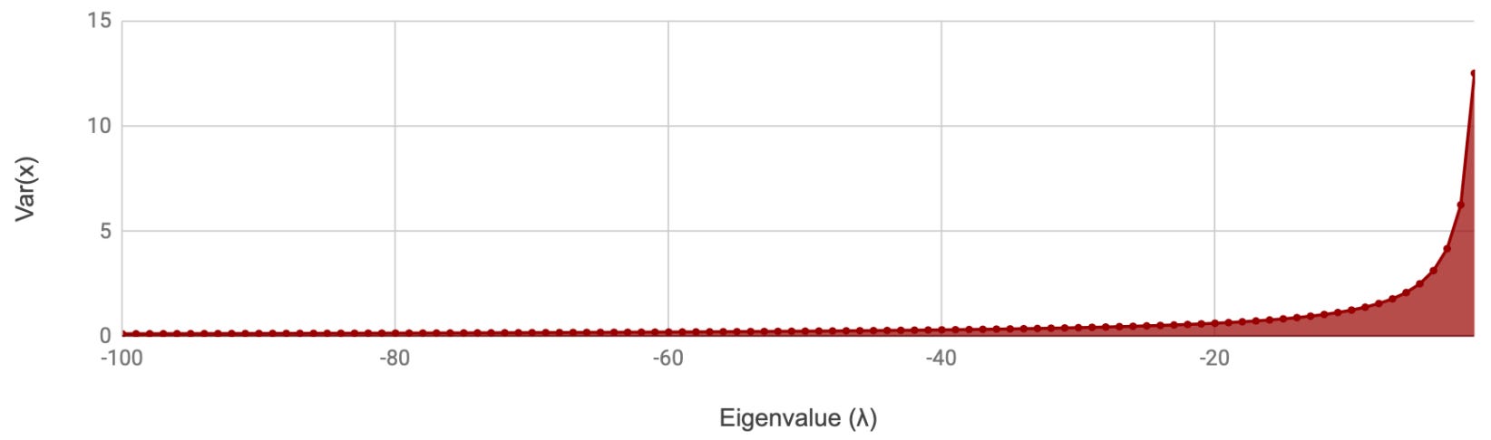
The steady-state variance of a system approaching a tipping point, Var(x), is given by the formula below where λ is the dominant eigenvalue of the system’s Jacobian matrix (where λ<0 for an equilibrium to remain stable) and σ2 represents the intensity of the background environmental noise or shocks. The following figure shows what happens when λ goes from -100→0, demonstrating how a weakening restoring force results in increased variance.
For more on this topic, see Issue № 83 // Spectral Deviation From Randomness.
Think of your original time series as the messy, fluctuating surface of the ocean. SSA and PCA act like a filter that splits this complex sea into individual, clean waves (eigenvectors) of different sizes. Big, powerful waves have large eigenvalues and hold most of the energy in the ocean. If you watch the water, these big waves control the main motion you see and feel. Small ripples (small eigenvalues), on the other hand, have very little energy and do not change the main flow of the sea. The full sea (total variance) represents the total energy of the whole ocean, which is the sum of all the big waves and small ripples (all eigenvalues) added together.
Choosing L requires balancing a strict trade-off between statistical power and stationary. If L is too short, the window will not capture long-term dynamics and the resulting estimates of variance and autocorrelation will be noisy and unstable. If L is too long though, the matrix will violate stationarity by blending distinct operational states together, inadvertently smoothing over the trends you’re trying to detect. Standard practices dictates setting the window length to 33% to 50% of the total time series length within that block (ex., L=8-12 for a 25-point block). In practice, we should run a sensitivity analysis with different window size percentages to ensure that detected signals remain consistent and are not artifacts of an arbitrary parameter choice.
If you’re having trouble following the linear algebra in this issue and want to learn more I strongly recommend Howard Anton’s Elementary Linear Algebra. I personally, found this book much more useful than Gilbert Strang’s textbooks / courses, which are more commonly recommended despite being much harder to follow imo.
When using PCA to detect signatures of criticality in multivariate data, we look for leading eigenvalues swelling beyond λmax (the maximum eigenvalue expected under a random noise matrix model); as discussed in Issue # 83. Similarly, when using SSA to detect CSD, we look for the leading eigenvalue of the lag-covariance matrix to explode across sequential time blocks.
You can generate the synthetic data from this example using the following code:
import numpy as np, pandas as pd
N_OBS, DT, SUBSTEPS, BURN = 1000, 1.0, 20, 500
OMEGA, ZETA_START, ZETA_END, SIGMA = 2*np.pi/30.0, 0.35, 0.02, 0.02
FAST, OBS_NOISE_SD, SEED = [(7.0, 0.16), (11.0, 0.11)], 0.05, 13
def simulate(zeta_path, omega=OMEGA, sigma=SIGMA, dt=DT, substeps=SUBSTEPS, rng=None):
    h, x, v = dt/substeps, 0.0, 0.0
    sh = np.sqrt(h); out = np.empty(len(zeta_path))
    for i, zeta in enumerate(zeta_path):
        for _ in range(substeps):
            dv = (-2*zeta*omega*v - omega**2*x)*h + sigma*sh*rng.standard_normal()
            x += v*h; v += dv
        out[i] = x
    return out
rng = np.random.default_rng(SEED)
zeta_ramp = np.r_[np.full(BURN, ZETA_START), np.linspace(ZETA_START, ZETA_END, N_OBS)]
zeta_flat = np.full(BURN + N_OBS, ZETA_START)
slow_csd  = simulate(zeta_ramp, rng=rng)[BURN:]
t = np.arange(N_OBS)*DT
fast = sum(a*np.sin(2*np.pi*t/p + rng.uniform(0, 2*np.pi)) for p, a in FAST)
df = pd.DataFrame({"t": t,"x_csd":  slow_csd  + fast + rng.normal(0, OBS_NOISE_SD, N_OBS)})
df = df.set_index('t')Another option here would be to use a high-pass Gaussian filter. This differs from the rolling mean subtractor in that it uses a weighted average based on a Gaussian distribution whereas a standard rolling mean uses a flat, equally-weighted window.
Here we’re using the non-parametric Pearson moment estimator, which directly calculates the standardized covariance between the time series and its self-shifted counterpart (xt and xt-1). This method is highly efficient for direct, fast computation using rolling window statistics. The alternative is the Autoregressive Model of Order 1, AR(1), estimated via ordinary least squares (OLS). While both methods yield the same mathematical coefficient value under stationarity the AR(1) OLS framework explicitly isolates environmental noise. This allows you to construct confidence intervals, perform tests for statistical significance, and simulate the system's future path.


